From the Circle to the Qubit: Understanding Relative Phase from First Principles

Relative phase is one of the most important ideas in quantum mechanics and quantum computing.

It is also one of the most frequently misunderstood.

The formula below is a preview of the destination. Its notation is not assumed here: every symbol and operation will be constructed before the formula is used in the quantum sections.

A qubit can be written as

where $\alpha$ and $\beta$ are generally complex numbers. Their magnitudes determine the probabilities associated with measurement, while the angular relationship between them—their relative phase—determines how the two components interfere.

That description is mathematically correct, but it can feel abstract if the ideas beneath it have not been built carefully.

What is a phase?

Why is phase represented by an angle?

Why do angles naturally lead to radians?

Why does the number $\pi$ appear?

Why do sine and cosine enter the description?

Why are complex numbers necessary?

And why can two quantum states have identical measurement probabilities in one basis while behaving completely differently after a quantum gate?

The answer begins not with quantum mechanics, but with one of the simplest objects in elementary geometry:

a circle.

From the distinction between linear and angular quantities, we can construct the concept of an angle. From the circle, we obtain $\pi$. From $\pi$, we obtain the radian. From the radian and the unit circle, we obtain sine and cosine. From sine and cosine, we obtain rotations and periodic motion. From rotations, we obtain phase. From phase, we obtain the complex exponential. And from the complex exponential, we arrive naturally at the relative phase of a qubit.

The path is longer than simply stating the final formula, but every step explains why the next one exists.

A note from the author

This article, and the articles that will follow it, are guided by a simple conviction: difficult ideas become clearer when they are encountered not as isolated results, but as parts of a connected structure. Mathematics and science are not a catalogue of formulas to be memorized. They are a network of relationships in which an elementary idea, understood precisely, can become the foundation of a much more advanced one.

I wrote this essay as a single, continuous path through concepts that are often separated across many chapters of a mathematics text: lengths and angles, circles and $\pi$, radians, trigonometry, complex numbers, waves, and finally quantum phase. The aim is not to make the subject artificially easy. It is to make its internal logic visible, so that each step has a reason to exist and the next step can feel like a consequence rather than a leap.

For some readers, the early sections may provide a first solid encounter with ideas that have previously seemed disconnected. For others, they may offer a chance to revisit familiar material and see how it supports quantum mechanics. Both readings matter. Prerequisites are not merely obstacles to clear; they are the conceptual bridges that make deeper understanding possible.

This is why the journey begins with a circle and reaches a qubit only gradually. A reader may pause, return, and move at a different pace through different sections. The goal is the same at every level: to replace a collection of separate facts with a coherent mental picture. That will remain the guiding principle of the articles to come.

1. Linear quantities and angular quantities

The first distinction we need is the difference between a linear quantity and an angular quantity.

A linear quantity measures displacement or extension along a path.

Examples include:

• the length of a table;
• the distance between two cities;
• the radius of a circle;
• the distance travelled by a car;
• the length of an arc.

Linear quantities are measured in units such as metres, centimetres, or kilometres.

If a point moves from $A$ to $B$ along a straight line, its displacement can be described by a length:

An angular quantity describes something different. It measures a change in direction around a reference point or axis.

Imagine a rigid hand attached to the centre of a clock. The tip of the hand moves along a curved path, but the most natural description of the hand's motion is not merely the distance travelled by its tip. It is the amount through which the entire hand has rotated.

That rotation is described by an angle.

Two clock hands of different lengths can rotate through exactly the same angle even though their tips travel different distances.

For example, suppose two radial segments have lengths $r_1$ and $r_2$, with

If both rotate through the same angle, the point at distance $r_2$ from the centre travels along a longer arc than the point at distance $r_1$.

The angular displacement is identical, but the linear displacement is not.

This distinction is essential:

A linear quantity describes how far a point travels, while an angular quantity describes how much a direction changes.

The two quantities are related, but they are not the same.

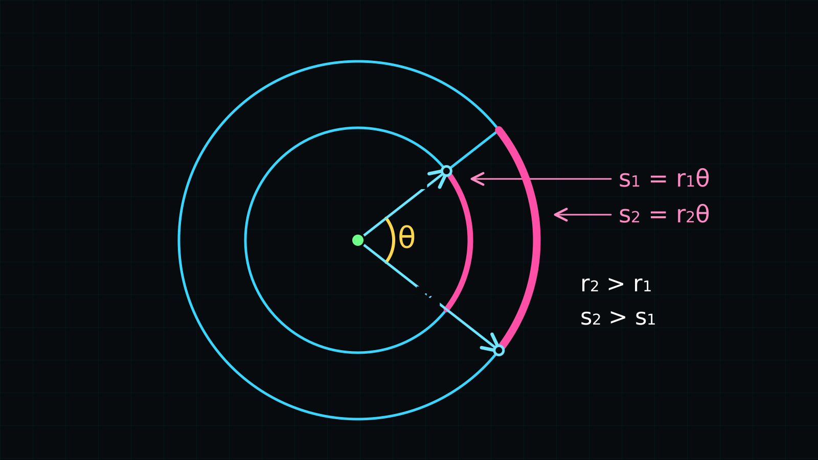
Caption: Two concentric circles with radii $r_1$ and $r_2$. Two radial lines form the same central angle $\theta$ on both circles. The outer arc is visibly longer than the inner arc, demonstrating that the same angular displacement can correspond to different linear distances.

2. What exactly is an angle?

An angle can be understood as the amount of rotation required to transform one direction into another.

Take two rays that begin at the same point. That common point is called the vertex.

If one ray is treated as the initial direction and the other as the final direction, the angle measures the rotation between them.

This definition is deeper than the common description of an angle as merely “the space between two lines.” An angle is fundamentally associated with rotation.

A full rotation returns a direction to its initial orientation.

A half rotation reverses the direction.

A quarter rotation produces a perpendicular direction.

Degrees provide one conventional way to divide a complete rotation:

Therefore,

and

The number $360$ is historically convenient, but it is not forced upon us by geometry itself. A complete rotation could have been divided into $100$, $400$, or $1000$ arbitrary units.

Radians are different.

The radian is not based on an arbitrary subdivision. It arises directly from the geometry of the circle.

To understand why, we first need to understand the number $\pi$.

3. The geometric meaning of $\pi$

Consider any circle.

Let

denote its radius,

its diameter, and

its circumference.

The diameter is twice the radius:

The constant $\pi$ is defined as the ratio between the circumference of a circle and its diameter:

Since

we can also write

Multiplying both sides by $D$, we obtain the familiar circumference formula:

Substituting

gives

The same relation can be rearranged to isolate $\pi$:

This equation explains the geometric meaning of $\pi$: it tells us how many diameter-lengths fit around the circumference of a circle.

Numerically,

The decimal expansion continues indefinitely without repeating periodically.

The crucial fact is that the ratio

is the same for every Euclidean circle, regardless of its size.

If the diameter doubles, the circumference doubles.

If the radius is multiplied by a factor $k$, then

and the new circumference becomes

The circle becomes larger, but its shape does not change. Therefore, the ratio between circumference and diameter remains constant.

That universal constant is $\pi$.

4. From circumference to arc length

A circumference is the total length around a circle.

An arc is only part of that circumference.

Suppose a central angle selects an arc of length

If the angle is a certain fraction of a complete rotation, then the selected arc is the same fraction of the full circumference.

For example, a half rotation selects half the circumference:

Since

we obtain

A quarter rotation selects one quarter of the circumference:

so

The length of an arc therefore depends on two things:

1. the amount of rotation;
2. the radius of the circle.

The same angle cuts a longer arc from a larger circle.

This is precisely where linear and angular quantities meet.

5. The natural definition of the radian

Suppose an angle cuts an arc of length $s$ from a circle of radius $r$.

Both $s$ and $r$ are lengths: they are linear quantities, even though the arc associated with $s$ is curved. In the International System of Units, the standard unit of length is the metre. The same lengths could also be expressed in centimetres, kilometres, or another suitable unit, provided that the same unit is used for both.

Why the length of a curved arc is still a linear quantity

The curved shape of an arc can make it seem angular, but its length answers a purely linear question: how long is this line when measured along its entire extent?

Imagine a flexible cord laid on a flat surface in the shape of a circle. The cord is curved, but its length can be found by straightening it without stretching it and then measuring it against a metre rule or measuring tape. Changing the cord from a circular shape into a straight one changes its direction at each point, but it does not change how long the cord is.

The circumference $C$ is precisely the total length of the curve forming a complete circle. As established above,

It is the length corresponding to the entire circular arc selected by a complete rotation of $360^\circ$. The same reasoning applies to a partial arc or to any other curved line: asking for its length means asking how far the line extends, not how much its direction changes.

What is angular is the change in direction of the radius, or equivalently the total turning of the tangent as one moves along the curve. Arc length and angular change are therefore related, but they are not the same kind of quantity.

With this distinction in place, the angle measured in radians is defined by

Equivalently,

This formula is one of the most important bridges between linear and angular measurement.

The numerator $s$ is the length of the arc.

The denominator $r$ is the length of the radius.

Because they are lengths expressed in the same unit, their units cancel in the ratio. If both are measured in metres, for example, metres cancel against metres. The numerical values of $s$ and $r$, however, do not disappear: what remains is the ratio $s/r$, which is not automatically equal to $1$.

An angle measured in radians is dimensionless in the formal dimensional-analysis sense. But “dimensionless” does not mean meaningless. The value $s/r$ still represents a geometrically meaningful ratio and therefore a specific amount of rotation.

One radian

An angle measures exactly one radian when the length of the intercepted arc equals the radius:

Substituting into

gives

Only in this particular case does the numerical ratio become $1$, because the two lengths are equal. Thus:

One radian is the angle that intercepts an arc whose length is equal to the radius of the circle.

This definition does not depend on the size of the circle.

For a small circle, both $s$ and $r$ are small.

For a large circle, both are large.

But if

their ratio is always

That is why the radian is a true angular measure rather than a linear one.

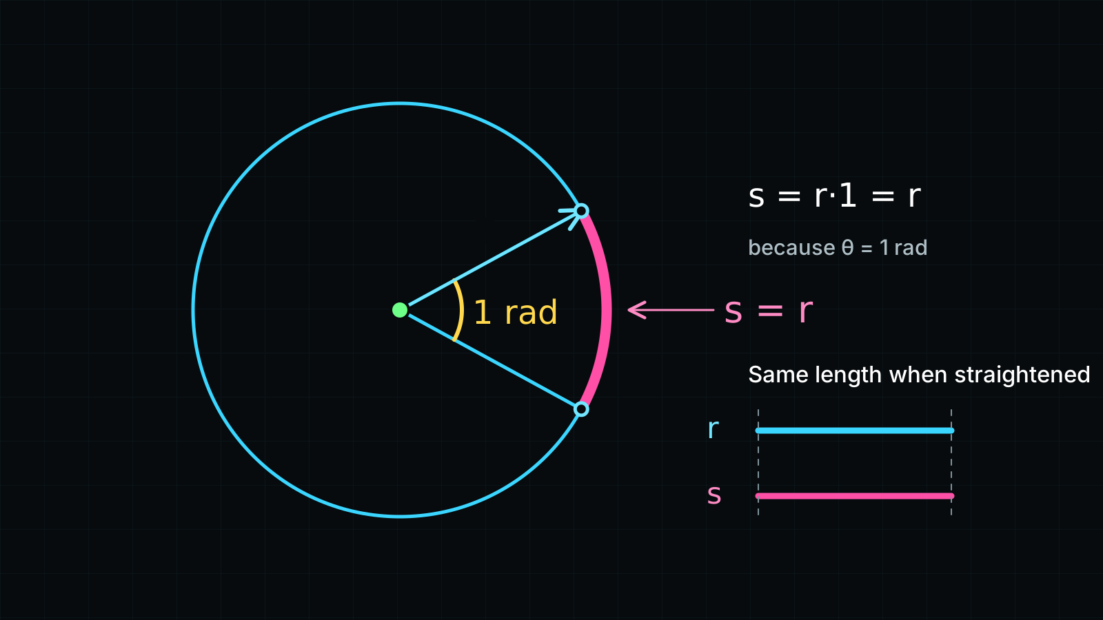
Caption: A circle of radius $r$ with a central angle of exactly $1$ radian, approximately $57.3^\circ$. Since $s=r\theta$, setting $\theta=1$ gives $s=r$. The equal-length segments on the right compare the radius with the same arc after it has been conceptually straightened.

6. Why a full circle contains $2\pi$ radians

For a complete rotation, the arc length is the entire circumference:

Since

the angular measure of a full rotation is

Therefore,

A half rotation is

and a quarter rotation is

The relationship between degrees and radians is therefore

which simplifies to

Consequently,

radians, while

Numerically,

Radians are natural because the number $2\pi$ is not imposed by convention. It follows directly from the ratio between the circumference and the radius:

The geometry of the circle itself tells us that a complete rotation contains $2\pi$ radians.

7. Why radians are more fundamental than degrees

Degrees are useful for everyday communication, but radians reveal the mathematical structure of rotation.

The arc-length equation in radians is simply

If the angle were expressed in degrees, an additional conversion factor would be necessary:

Radians eliminate that artificial factor.

They also make the fundamental derivatives of trigonometric functions take their simplest form:

and

These identities are exactly true in this form only when $\theta$ is measured in radians.

Radians are therefore not merely an alternative notation. They are the angular units naturally selected by geometry, calculus, wave mechanics, and quantum theory.

8. The unit circle

The next step is to choose a circle whose radius is

This is called the unit circle.

For a general circle, arc length and angle are related by

On the unit circle the radius is

and therefore

This is an extraordinary simplification:

On the unit circle, the numerical value of an angle in radians is equal to the length of the arc it intercepts.

An angle and an arc length are still conceptually different quantities, but on the unit circle they have the same numerical value.

The unit circle is centred at the origin of a Cartesian coordinate system and has equation

Take the point

as the starting position and rotate counterclockwise through an angle $\theta$.

The resulting point on the unit circle is

This gives the geometric definitions of cosine and sine:

Cosine is the horizontal coordinate of the rotating point.

Sine is the vertical coordinate.

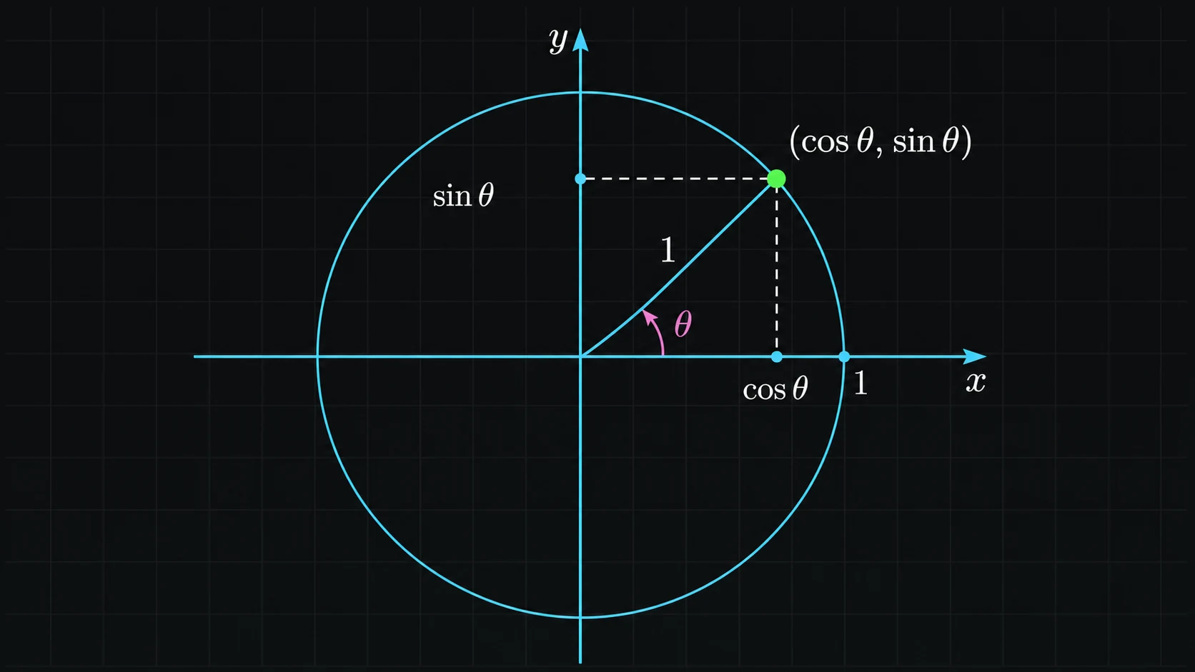
Caption: A unit circle centred at the origin. A radius forms an angle $\theta$ with the positive horizontal axis and reaches the point $(\cos\theta,\sin\theta)$. Dashed projections onto the axes show that the horizontal coordinate is $\cos\theta$ and the vertical coordinate is $\sin\theta$.

The tangent is defined whenever the cosine of $\theta$ is nonzero. This restriction is necessary because cosine appears in the denominator. The tangent is then given by

It can also be interpreted geometrically as the slope of the radial line:

There is also a classical construction that explains the name. The vertical line $x=1$ is tangent to the unit circle at $A=(1,0)$. Extending the radial line at angle $\theta$ until it meets this tangent line gives the point

Thus the signed vertical segment from $A$ to $T$ has length $\tan\theta$. This construction connects the ratio $\sin\theta/\cos\theta$, the slope of the radial line, and the geometric tangent to the circle.

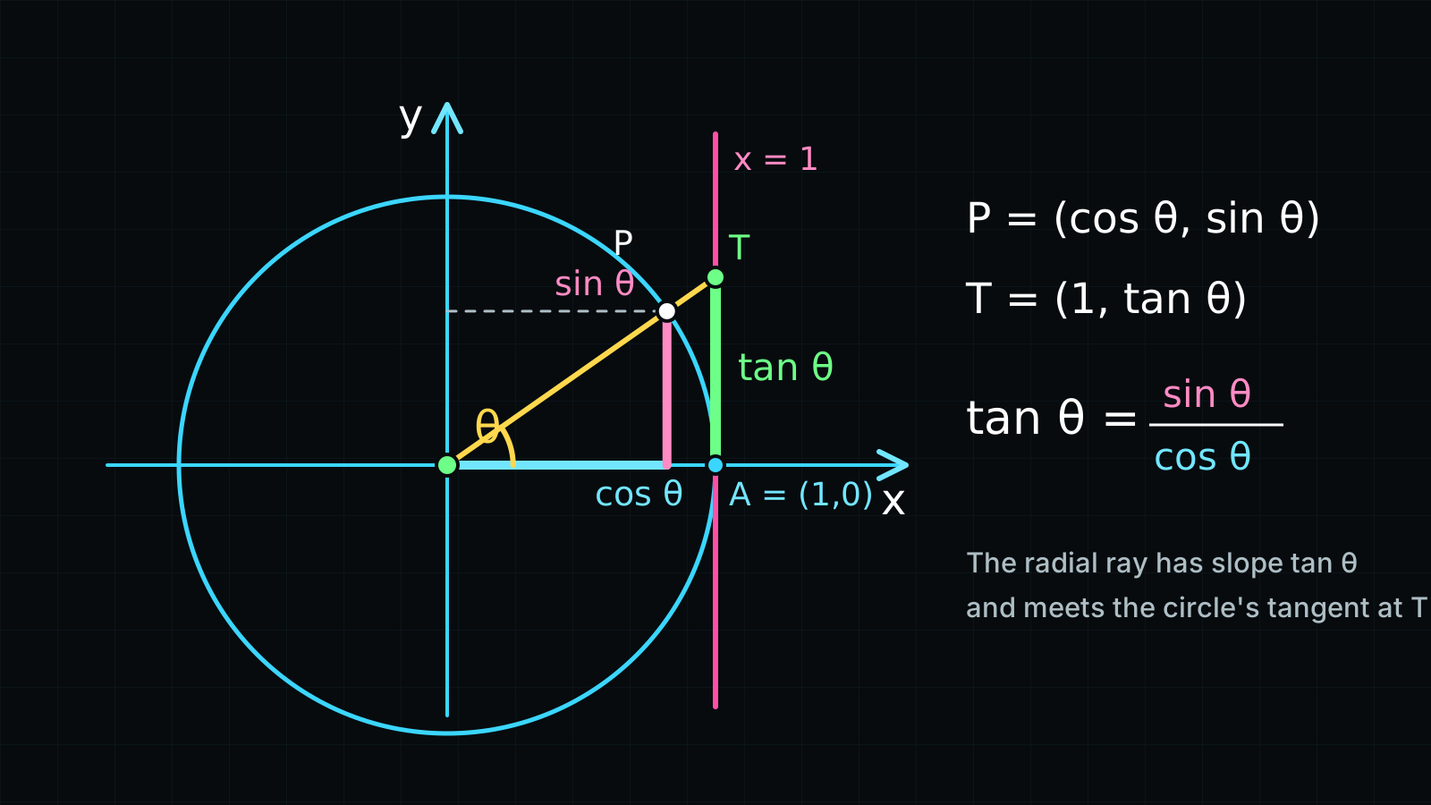
Caption: The point $P=(\cos\theta,\sin\theta)$ lies on the unit circle. Its radial line has slope $\tan\theta=\frac{\sin\theta}{\cos\theta}$ and meets the tangent line $x=1$ at $T=(1,\tan\theta)$. The vertical segment from $A=(1,0)$ to $T$ therefore represents $\tan\theta$.

Thus trigonometry is not a disconnected collection of formulas. It is the coordinate geometry of rotation around the unit circle.

9. Sine and cosine as records of rotation

Imagine a point moving around the unit circle at a constant angular rate.

Its horizontal coordinate changes as

while its vertical coordinate changes as

As the point completes one full rotation, the values repeat:

Sine and cosine are therefore periodic functions with period

This periodicity is not an arbitrary algebraic feature. It reflects the fact that rotating by an additional full turn returns the point to the same position.

For example,

After one full rotation,

The point has returned to its starting location.

A phase angle will later tell us where a periodic system is located within such a cycle.

10. From angle to phase

The word phase describes a position within a repeating cycle.

Consider two oscillations:

and

Both have amplitude $A$ and angular frequency $\omega$, but the second contains an additional angle $\phi$.

Angular frequency tells us how quickly the phase advances through a cycle. It is an angle accumulated per unit time, so its natural unit is radians per second:

The variable $t$ represents a time interval and is measured in seconds. Consequently, the product $\omega t$ has units of radians for every value of $t$:

Thus $\omega t$ is itself an angle and is therefore a valid argument of the cosine. Its numerical value at any chosen time $t$ gives the phase accumulated since the selected starting time. Mathematically an angle is a dimensionless scalar (the radian is the ratio of arc length to radius), while writing it in radians keeps its angular meaning explicit.

The evolving phase $\omega t$ is common to both oscillations. The additional angle $\phi$, not $\omega t$, is the constant phase offset of the second oscillation relative to the first.

If

the oscillations reach their maxima and minima together. They are said to be in phase.

If

then

so one oscillation reaches its maximum when the other reaches its minimum. They are in opposite phase.

If

one oscillation is shifted by one quarter of a cycle.

Because a full cycle corresponds to

phase is naturally an angular quantity.

The value of $\phi$ does not describe a physical distance. It describes displacement within a cycle.

This is why phase is measured in radians.

11. Relative phase in ordinary waves

To understand why relative phase matters, consider two waves with the same amplitude and frequency:

Their sum depends on $\phi$.

When

we obtain

The waves reinforce each other. This is constructive interference.

When

we obtain

and therefore

The waves cancel. This is destructive interference.

The individual amplitudes have not changed. What changed is their angular relationship.

This is the core meaning of relative phase:

Relative phase measures the angular difference between components that can interfere.

Only the difference is important.

If both waves are shifted by the same phase $\gamma$,

their relative phase remains

The common phase $\gamma$ changes the shared reference, but it does not change the relationship between the waves.

This distinction between common phase and relative phase will reappear in the quantum description of a qubit.

12. Why complex numbers enter the picture

A point on the unit circle can be represented by its Cartesian coordinates:

The same point can be encoded as a complex number, conventionally denoted by $z$:

where the imaginary unit satisfies

Euler's formula states that

This identity follows directly from the Maclaurin series. For every real number $x$,

while

and

Now substitute $x=i\phi$ into the exponential series. Since $i^2=-1$, its even powers become real alternating terms and its odd powers become $i$ times real alternating terms:

The first parenthesis is $\cos\phi$; the second is $\sin\phi$. Hence $e^{i\phi}=\cos\phi+i\sin\phi$. This is not a convention or an analogy: the complex exponential and the trigonometric form are exactly the same number, written in two equivalent ways.

Therefore, a unit complex number can be written compactly as

This is not merely a symbolic trick.

The complex exponential represents a rotation through an angle $\phi$ in the complex plane.

Multiplication by

rotates a complex number through the angle $\phi$ without changing its magnitude.

For example,

and

These values correspond to one complete journey around the unit circle in the complex plane.

More generally, a complex number can be written in polar form as

where

is its magnitude and $\phi$ is its phase.

The words magnitude and modulus refer to the same quantity.

If

then its magnitude is the ordinary Euclidean distance from the point $(x,y)$ to the origin of the complex plane:

In polar form this becomes

We will also need the complex conjugate. For

its conjugate is written with an asterisk:

Geometrically, conjugation reflects the point across the real axis. Multiplying a complex number by its conjugate removes the imaginary part:

For the polar form,

Using Euler's formula,

A complex number therefore contains two independent pieces of information:

1. a magnitude $\rho$;
2. an angle $\phi$.

That angle is the complex phase.

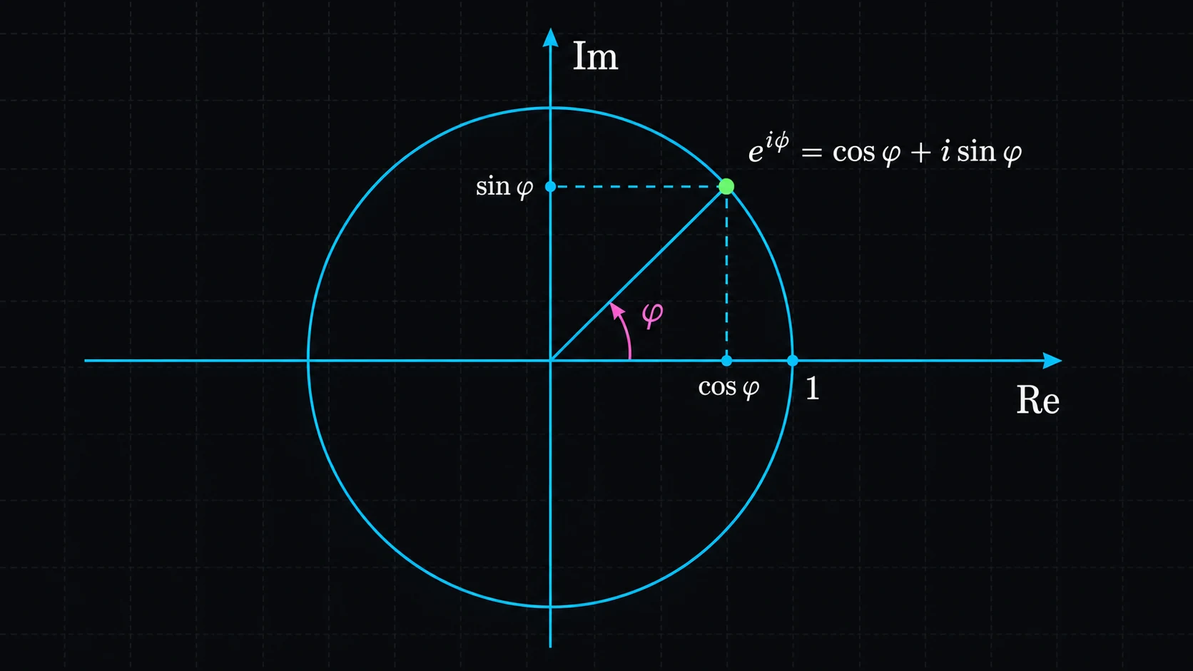
Caption: The complex plane with a unit vector from the origin to the point $e^{i\phi}=\cos\phi+i\sin\phi$. The horizontal axis represents the real component, the vertical axis the imaginary component, and the angle $\phi$ is measured counterclockwise from the positive real axis.

Complex numbers are useful here because one number can carry both a magnitude and an angle. Quantum mechanics needs precisely that combination: magnitudes will determine probabilities, while angular relationships will determine interference. This is why the next step introduces complex amplitudes rather than ordinary probabilities alone.

13. Complex amplitudes in quantum mechanics

In classical probability theory, probabilities are represented by non-negative real numbers.

Quantum mechanics works differently.

Quantum states are described by complex probability amplitudes.

Before using those amplitudes, we need a small amount of vector language. A pure state is the most specific state description quantum mechanics allows for an individual system. For a qubit, it is written

and the symbol $|\psi\rangle$ is read ket psi. A ket represents a vector in the complex state space of the quantum system.

To describe a vector, we first choose a basis: a set of independent reference directions from which every vector in the space can be constructed. For a qubit, the standard choice is the computational basis

The kets $|0\rangle$ and $|1\rangle$ are basis vectors, not the ordinary numerical values zero and one. After this basis has been chosen, they can be represented by the coordinate columns

The complete state is therefore represented in this basis by

where

The amplitudes $\alpha$ and $\beta$ are the complex coordinates of the state relative to the chosen basis. The abstract ket and its coordinate column are closely related but are not identical concepts: the column is the representation of the ket after a basis has been selected.

The state space is called two-dimensional because two independent basis directions are required. Each coordinate is complex, so this is not an ordinary two-dimensional real plane. It is the complex vector space $\mathbb{C}^2$. More precisely, it is a Hilbert space: a complex vector space equipped with the mathematical structure needed to define lengths, angles, orthogonality—the generalization of perpendicular directions—and probabilities.

The two basis vectors represent two distinguishable quantum alternatives. Depending on the physical system, they might represent:

• two spin states of an electron;
• two polarization states of a photon;
• two energy levels of an atom;
• two possible paths through an interferometer;
• two states of a superconducting circuit.

A fundamental particle is not automatically “a qubit” in every circumstance. A qubit is obtained when we identify and control a two-dimensional quantum degree of freedom.

Measuring in the computational basis is a physical operation whose possible outcomes are associated with $|0\rangle$ and $|1\rangle$. It asks which of those two basis alternatives is obtained. The amplitudes $\alpha$ and $\beta$ are not themselves measurement outcomes, and measurement does not merely read the entries of a column.

Instead, the probabilities are obtained from the squared magnitudes of the amplitudes:

Because one of the two possible outcomes must occur, their probabilities must sum to one. The state therefore satisfies the normalization condition

The word normalization means that the total probability has been scaled to one. Since the magnitude of a complex number is its distance from the origin, the squared magnitudes are non-negative real numbers and can consistently serve as probabilities.

Consider one elementary example:

so the computational-basis outcomes are equally probable. The notation $\arg(w)$ denotes the phase angle, or argument, of a complex number $w$. Here,

and therefore the relative phase of the second amplitude with respect to the first is

The state is

When the Bloch sphere is introduced later, this state will appear on its equator in the $+y$ direction. This single example already joins magnitude, probability, complex argument, and relative phase.

At first sight, the probability rule might suggest that only the magnitudes of $\alpha$ and $\beta$ matter.

But that conclusion would be incomplete.

The phases of the amplitudes determine how the two components interfere under other measurements or quantum transformations.

14. Separating magnitude and phase

Every non-zero complex amplitude can be written in polar form.

Let

and

where $a$ and $b$ are phase angles.

Equivalently,

The qubit state becomes

We can factor out the common phase $e^{ia}$:

Define

Then

This expression reveals two different kinds of phase:

• the factor $e^{ia}$, which multiplies the entire state;
• the phase difference $\phi=b-a$, which exists between the two basis components.

The first is called a global phase.

The second is called a relative phase.

15. Global phase

Suppose we multiply the entire quantum state by

Then

If

then

The measurement probabilities in the computational basis are unchanged because

Since

we have

Similarly,

More generally, all predictions for an isolated pure state remain unchanged by a global phase.

Therefore,

and

represent the same physical pure state.

A global phase changes the mathematical representative of the state vector but not the physical state represented by that vector.

16. Relative phase

Now consider the state

The factor

multiplies only the $|1\rangle$ component.

It therefore changes the angular relationship between the two components.

That relationship cannot be removed by multiplying the entire state by one common phase.

The angle $\phi$ is the relative phase.

Two states can have the same computational-basis probabilities while having different relative phases.

For example, consider

and

For $|+\rangle$, the relative phase is

For $|-\rangle$, the minus sign can be written as

so the state can be written as

Its relative phase is therefore

If either state is measured directly in the computational basis,

and

The two states appear identical under that particular measurement.

Yet they are not the same state.

Their different relative phases produce different interference behaviour.

17. Turning relative phase into a measurable probability

A phase is not measured by reading an invisible angular label attached to a particle.

Instead, quantum operations convert phase differences into differences in measurement probability.

A single-qubit quantum gate is a linear transformation of the state vector. After the computational basis has been chosen, the gate can be represented by a $2\times2$ complex matrix. Physical gates for an isolated qubit are unitary transformations, meaning that they preserve normalization and therefore preserve total probability.

Linearity means that for any complex numbers $c_0$ and $c_1$,

This is why knowing what a gate does to the two basis vectors determines what it does to every qubit state.

The Hadamard gate is a simple and especially important example:

The two columns of this matrix are the coordinate representations of $H|0\rangle$ and $H|1\rangle$. They encode

and

Applying the Hadamard gate to $|+\rangle$ gives

Applying it to $|-\rangle$ gives

Before the Hadamard gate, both states produced $0$ and $1$ with equal probability in the computational basis.

After the Hadamard gate, they become perfectly distinguishable.

The relative phase has been transformed into a population difference, meaning a difference between the probabilities associated with the two basis states.

This is quantum interference.

18. A general relative-phase experiment

Consider the balanced qubit state

The computational-basis probabilities are

and

for every value of $\phi$.

A direct computational-basis measurement therefore reveals nothing about the relative phase.

Now apply a Hadamard gate:

Substituting the action of $H$,

Collecting the coefficients of $|0\rangle$ and $|1\rangle$,

The probability of measuring $0$ is

From the conjugation rule introduced earlier,

Using $|z|^2=z\,z^*$, we therefore obtain

Expanding,

Since

we have

Therefore,

Using the half-angle identity,

so

Similarly,

The final measurement probabilities therefore depend directly on the relative phase:

Several important cases follow immediately.

If

then

If

then

If

then

This calculation captures the operational meaning of relative phase:

Relative phase affects observable results when quantum components are recombined so that they can interfere.

19. The Bloch-sphere representation

Before introducing the sphere, three different mathematical objects must be kept separate.

The complex plane $\mathbb{C}$. One complex amplitude, such as $\alpha$ or $\beta$, can be represented by one point or vector in the complex plane.

The qubit Hilbert space $\mathbb{C}^2$. The complete qubit state is the ordered pair

It belongs to a two-dimensional complex vector space, not to an ordinary two-dimensional real plane. As introduced earlier, calling this space a Hilbert space means that it also has the structure needed to define lengths, orthogonality, and probabilities.

The Bloch sphere. The sphere is not literally the full Hilbert space. It is a three-dimensional geometric representation of the physically distinct normalized pure states after the global phase has been removed.

In short: one amplitude lives in $\mathbb{C}$, the complete ket lives in $\mathbb{C}^2$, and the corresponding physical pure state can be represented by one point on the Bloch sphere.

Every pure qubit state can be written, up to an irrelevant global phase, as

In the standard convention, the two parameters are restricted to

Angle and phase are not synonyms

The parameters $\theta$, $\phi$, and, when it is retained, $\gamma$, are all angular quantities measured in radians. They nevertheless play different mathematical roles.

The parameter $\gamma$ is a global phase when it appears in the unit-modulus factor $e^{i\gamma}$ multiplying the entire ket. The parameter $\phi$ is a relative phase because it appears in $e^{i\phi}$ and expresses the difference between the complex arguments of the two amplitudes:

By contrast, $\theta$ is a polar angle, not a phase. It appears in the real quantities that determine the magnitudes of the amplitudes:

It therefore controls the probability distribution in the computational basis,

whereas $\phi$ controls the relative complex orientation of the two components and can therefore affect interference.

Euler's formula makes the distinction explicit:

The factor $e^{i\phi}$ has unit modulus; changing $\phi$ changes its argument in the complex plane without changing that modulus. This is what makes $\phi$ a phase. Every phase is represented by an angle, but not every angle is a phase: an angle is called a phase when it describes the argument of a complex quantity, as in $e^{i\phi}$, or a position in a periodic cycle. The angle $\theta$, even though it appears in trigonometric functions, parametrizes real amplitude magnitudes and the north-south position on the Bloch sphere.

This is the standard Bloch-sphere representation. Its corresponding point has coordinates

At fixed $\phi$, varying $\theta$ moves the point along a meridian and changes the weights of $|0\rangle$ and $|1\rangle$. At fixed $\theta$, varying $\phi$ rotates the point around the $z$-axis while leaving the computational-basis probabilities unchanged. A global phase $\gamma$ produces no displacement on the Bloch sphere, because it does not distinguish a physically different pure state.

The computational basis states lie at the poles:

Balanced superpositions lie on the equator, where

For example,

corresponds to

while

corresponds to

Other equatorial states include

with

and

with

Moving around the equator changes the relative phase while keeping the computational-basis probabilities fixed at

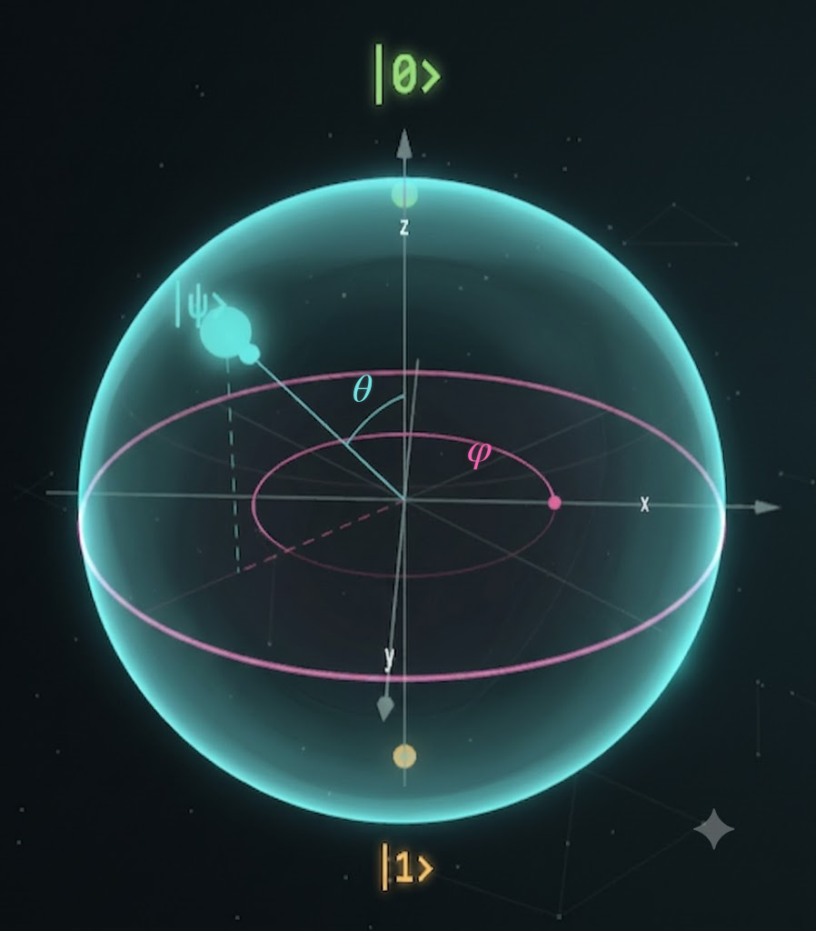
Caption: A Bloch sphere showing $|0\rangle$ at the north pole, $|1\rangle$ at the south pole, and the states $|+\rangle$, $|+i\rangle$, $|-\rangle$, and $|-i\rangle$ around the equator. The polar angle $\theta$ represents amplitude balance, while the azimuthal angle $\phi$ represents relative phase.

20. Why the qubit formula contains half-angles

The appearance of

in

may seem surprising.

Why does the state use half of the Bloch-sphere polar angle?

The most direct answer comes from the probabilities. The two amplitudes give

The vertical Bloch coordinate records the imbalance between those probabilities:

Therefore,

This trigonometric identity explains directly why the amplitudes contain $\theta/2$ while the Bloch-sphere coordinate contains $\theta$.

At

we have $P(0)=1$, which gives the north pole. At

we have $P(1)=1$, which gives the south pole. At

both probabilities equal $1/2$, which gives the equator.

There is also a deeper structural explanation. A normalized two-component quantum state is a type of mathematical object called a spinor. It belongs to a complex vector space, while the Bloch vector is an ordinary three-dimensional real direction. The mapping between them is not one-to-one at the level of raw state vectors because

and

represent the same physical state.

In particular,

and

differ by the global phase

and therefore represent the same physical qubit state.

This produces a double-cover relationship: two state vectors that differ only by a sign correspond to the same physical Bloch-sphere point. This is the deeper rotation structure behind the half-angle.

A qubit state vector may acquire a minus sign after a physical rotation of

while returning exactly to its original vector only after a rotation of

The minus sign after a $2\pi$ rotation is a global phase for an isolated state, but it can become observable when compared interferometrically with a reference path that was not rotated.

This is one of the places where the apparently elementary geometry of angles leads into the deeper structure of spin-$\tfrac{1}{2}$ quantum systems.

21. Relative phase is not a tiny object physically rotating

It is important not to interpret quantum phase too literally.

When a qubit amplitude contains

this does not necessarily mean that a microscopic object is physically spinning around a visible circle in ordinary space.

The circle often belongs to an abstract mathematical space.

For a complex amplitude, phase is an angle in the complex plane.

For a qubit, relative phase describes the angular relationship between complex amplitudes associated with different basis states.

The physical implementation may involve:

• spin;
• polarization;
• energy;
• path;
• electric charge configurations;
• collective superconducting variables.

The mathematical phase is common to all these systems even though their physical mechanisms are different.

The circle is therefore not always a literal trajectory. It is the geometry of the state description.

22. Phase gates

Quantum computers manipulate relative phase directly.

A general single-qubit phase gate can be written as

Applied to the state

it produces

The $|0\rangle$ amplitude is unchanged, while the phase of the $|1\rangle$ amplitude increases by $\lambda$.

If

and

the initial relative phase is

After the gate, the phase of the second amplitude becomes

so the new relative phase is

The gate changes relative phase without directly changing the computational-basis probabilities:

and

remain the same.

Yet the state has changed, because its future interference behaviour has changed.

Important special cases include the $Z$ gate:

the $S$ gate:

and the $T$ gate:

Each gate introduces a specific angular shift between the basis components.

23. Phase accumulation during time evolution

Relative phase is not introduced only by gates. It also arises naturally during time evolution.

An energy eigenstate is a quantum state with a definite energy value. In the example below, $E_0$ and $E_1$ are the energies associated with the basis states $|0\rangle$ and $|1\rangle$. The symbol

denotes the reduced Planck constant.

According to the Schrodinger equation, a component with definite energy $E$ accumulates the phase factor

during a time interval $t$. We do not need the full differential equation here, but the phase law is a consequence of that equation rather than an independent assumption.

The product $Et$ has the dimensions of energy multiplied by time, the same dimensions as $\hbar$. Their ratio

is therefore dimensionless and can serve as an angular phase measured in radians.

Suppose $|0\rangle$ and $|1\rangle$ are energy eigenstates with energies $E_0$ and $E_1$.

An initial state

evolves as

Factor out the common phase

The factor outside the brackets is a global phase.

The physically relevant relative phase evolves as

Defining the energy difference

we have

The corresponding angular frequency is

Thus,

This shows a profound connection:

Energy differences generate the time evolution of relative phase.

Absolute energy contributes a common phase, while differences in energy generate observable relative motion in quantum-state space.

This is closely related to the general principle that observable physics depends on differences and relationships rather than on an arbitrary absolute phase reference.

24. Relative phase and quantum interference

Quantum algorithms depend not only on creating superpositions but on controlling their phases.

Consider a state containing many computational alternatives:

A useful quantum algorithm manipulates the amplitudes so that incorrect alternatives interfere destructively while desired alternatives interfere constructively.

The final probability of an outcome depends on the squared magnitude of the total amplitude leading to it.

If two computational paths contribute amplitudes $a_1$ and $a_2$, the combined probability is

Expanding,

so

The last two terms are interference terms.

If

and

where

are the non-negative magnitudes of the two contributions.

then

Throughout this article, relative phase is defined as the phase of the second component minus the phase of the first:

The algebra above naturally produces the reversed order, but cosine is an even function:

The observable interference is therefore unchanged by that reversal, even though the definition of $\Delta\phi$ itself retains a fixed order.

Therefore,

The interference depends on the relative phase $\Delta\phi$.

If

then

and the interference is maximally constructive.

If

then

and the interference is destructive.

The same trigonometric function that describes the horizontal coordinate of a point on the unit circle controls the interference of quantum amplitudes.

That is not a coincidence. Both phenomena arise from the geometry of phase.

25. A practical analogy: two clock hands

A useful analogy is to imagine two clock hands rotating at the same angular speed.

The absolute orientation of each hand may depend on how the clock was initially positioned. But the difference between their orientations tells us how they are related.

If the first hand has angle

and the second has angle

their relative angle is

Rotating the entire clock by an angle $\gamma$ changes both orientations:

But their difference remains

The common rotation is analogous to a global phase.

The angular separation is analogous to relative phase.

The analogy is not a complete model of quantum mechanics, but it accurately captures why a shared phase can be irrelevant while a phase difference can remain physically meaningful.

26. What can and cannot be observed

The following distinction is fundamental.

For an isolated pure state, a global phase

does not change observable predictions.

A relative phase between coherent alternatives can change observable predictions through interference.

The word coherent matters.

Coherence means that the relative phase between the components is sufficiently well defined and stable for the interference terms to survive. Relative phase can influence an experiment only while that relationship is preserved.

Interactions with uncontrolled environmental degrees of freedom can destroy that stability. This loss of coherence is called decoherence.

When coherence is lost, interference terms become suppressed, and the system begins to behave more like a classical statistical mixture.

A coherent superposition such as

contains a definite relative phase.

A classical mixture in which the system is in $|0\rangle$ half the time and $|1\rangle$ half the time does not contain the same phase relationship.

That mixture is not represented by one ket of the form

It represents ordinary uncertainty about which basis state is present, with no definite phase relationship between the alternatives.

Both produce

under direct computational-basis measurement, but only the coherent superposition can produce phase-dependent interference.

This is one of the clearest mathematical differences between quantum superposition and ordinary uncertainty.

27. The complete conceptual chain

We can now summarize the entire progression.

Step 1: Linear measurement

A length measures extension or displacement along a path.

Examples include the radius $r$, arc length $s$, and circumference $C$.