
By EntangledMind
What Does “Fundamental” Mean?
When physicists call a particle fundamental, they are making a statement about the current depth of experimental knowledge. A fundamental, or elementary, particle is one for which no internal structure has yet been detected. It is not presently understood as being made from smaller constituents.
A composite particle, by contrast, is a bound state of more elementary components. A proton is composite because it contains quarks and gluons. An atomic nucleus is composite because it contains protons and neutrons. An atom is composite because it contains a nucleus and electrons.
This distinction is empirical rather than metaphysical. To say that an electron is elementary does not prove that it must remain indivisible in every future theory. It means that experiments have found no electron radius, internal constituents, or substructure down to the smallest distances currently accessible.
The hierarchy of ordinary matter can therefore be sketched as follows:
- molecules are built from atoms;
- atoms contain electrons and nuclei;
- nuclei contain protons and neutrons;
- protons and neutrons are hadrons made from quarks and gluons;
- electrons and quarks are presently classified as elementary.
This hierarchy is useful, but it can also encourage a misleading picture in which nature is imagined as a collection of progressively smaller solid balls. Modern particle physics replaces that classical image with a more subtle framework: quantum field theory.
From Classical Particles to Quantum Fields
In classical mechanics, a particle is often idealized as a point with a definite position and momentum. It follows a trajectory through space, and forces alter that trajectory.
Quantum theory does not preserve this picture unchanged. A quantum object can be described by a state that assigns amplitudes to different possible measurement outcomes. Position and momentum cannot generally possess arbitrarily precise simultaneous values, and a particle can produce interference even when emitted one at a time.
Quantum field theory goes further. Its basic entities are fields extending throughout space and time. The electron field, photon field, quark fields, gluon field, and Higgs field are not confined to the locations where particles are detected. They are parts of the physical structure used to describe every region of spacetime.
A particle is then understood as a quantized excitation of an appropriate field. An electron is an excitation of the electron field. A photon is an excitation of the electromagnetic field. A Higgs boson is an excitation of the Higgs field.
The familiar analogy is a vibrating medium: a field is compared to an extended surface, while particles are compared to localized packets of vibration. The analogy is helpful, but incomplete. Quantum fields are not known to be mechanical substances vibrating inside a deeper material medium. Their excitations obey quantum superposition, relativistic causality, and particle-creation rules that have no exact classical counterpart.
The word quantized means that a field does not exchange energy in arbitrarily divisible amounts in every physical process. Its allowed excitations come in discrete units associated with particles. These excitations can be created and destroyed, provided that the relevant conservation laws are respected.
This is why particle physics naturally allows processes such as an electron and a positron annihilating into photons. The particles are not indestructible beads. They are states of quantum fields, and interactions can transfer energy and quantum numbers from one set of field excitations to another.
Even the idea of a fixed particle number is therefore not universal. A low-energy experiment may contain a well-defined number of electrons, but a sufficiently energetic interaction can create additional particle-antiparticle pairs. Quantum field theory is built to describe this changing particle content.
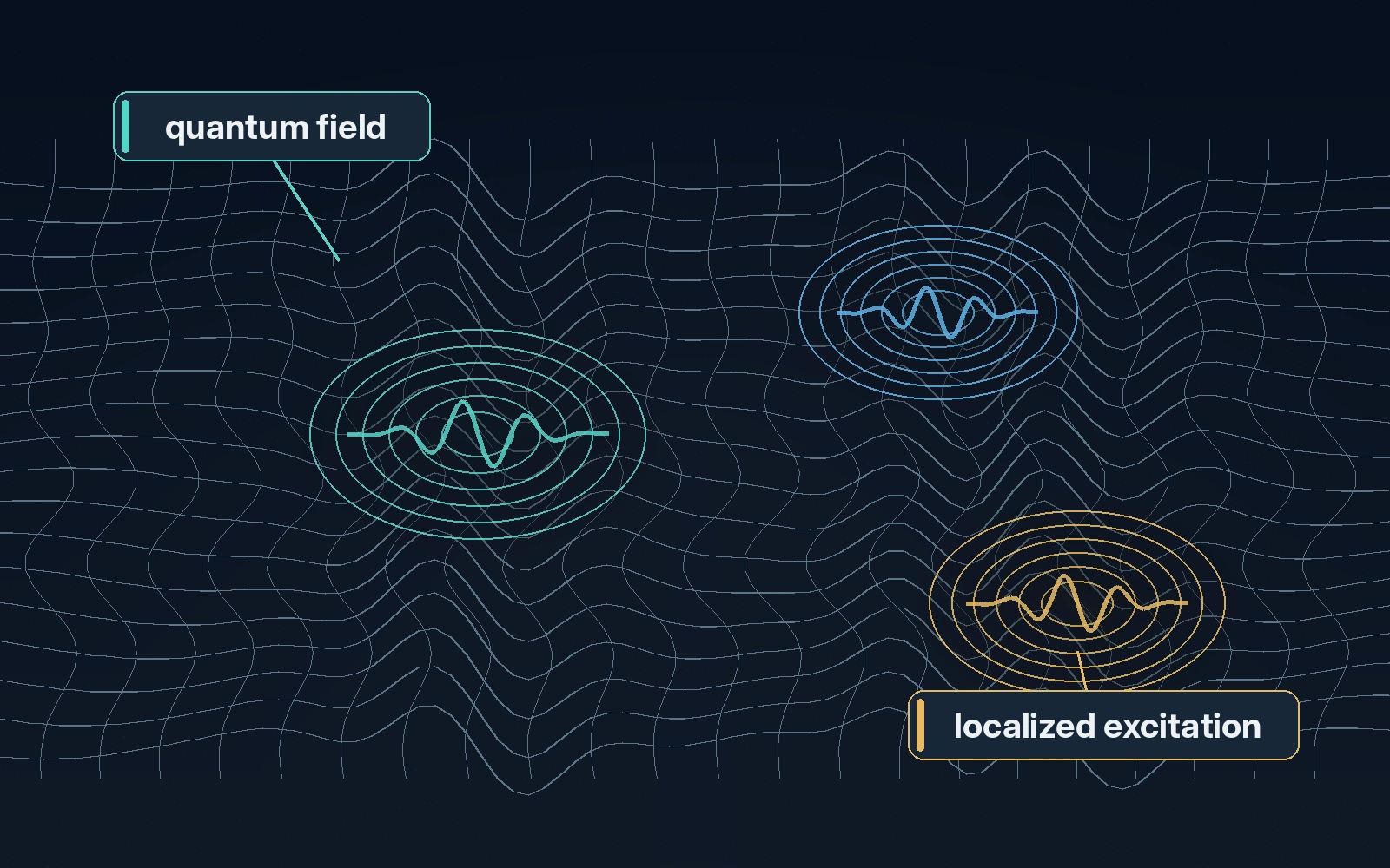
Caption: Quantum fields extend throughout spacetime; a particle is a localized, quantized excitation of one of those fields, not a tiny classical object.
Energy, Mass, Momentum, and Quantum Numbers
A particle species is not identified merely by its mass. It is characterized by a collection of measurable properties, including mass, spin, electric charge, colour charge, and its behaviour under the fundamental interactions.
Relativity connects a particle’s energy, momentum, and rest mass through
Here, is total energy, is the magnitude of momentum, is rest mass, and is the speed of light.
For a particle at rest, , so the relation becomes . A massless particle instead satisfies and cannot be brought to rest in an inertial frame.
Mass is therefore not simply “the amount of matter” inside an object. In modern physics, it is an invariant property of a state, connected to the relation between energy and momentum. Composite objects also possess mass, but their mass need not equal the simple sum of the rest masses of their constituents. Internal motion and interaction energy contribute to the total.
Particles also carry quantum numbers. These are labels associated with measurable properties and symmetry principles. Electric charge determines how a particle participates in electromagnetism. Colour charge governs participation in the strong interaction. Spin controls how a particle transforms under rotations and helps determine its quantum statistics.
Some quantum numbers are exactly conserved in known interactions. Others are conserved only under particular interactions or approximately under limited conditions. The Standard Model organizes these properties systematically rather than treating them as an unrelated catalogue.
Spin, Fermions, Bosons, and Exchange Symmetry
Spin is intrinsic angular momentum
Every elementary particle has a property called spin. Spin behaves mathematically like angular momentum, but it should not be pictured as a tiny solid sphere rotating around an axis.
A classical rotating charged object would need an extended surface and, for sufficiently small dimensions, could require parts of that surface to move faster than light. No such classical model correctly reproduces the observed properties of electrons or other elementary particles.
Spin is instead intrinsic. It is built into the way a quantum state transforms under spatial rotations and, more deeply, under the symmetries of relativistic spacetime.
Spin is measured in units of the reduced Planck constant . Particle physicists usually state only the dimensionless spin number. Electrons and quarks have spin . Photons and gluons have spin . The Higgs boson has spin .
This leads to the primary division of known particles:
- fermions have half-integer spin, such as ;
- bosons have integer spin, such as , , or .
The distinction is not merely terminological. Spin is connected to the behaviour of systems containing identical particles. Before that connection can be made precise, however, we need a small amount of mathematical language: what a quantum state is, how an observable acts on it, and what it means for a state to be an eigenstate of an observable.
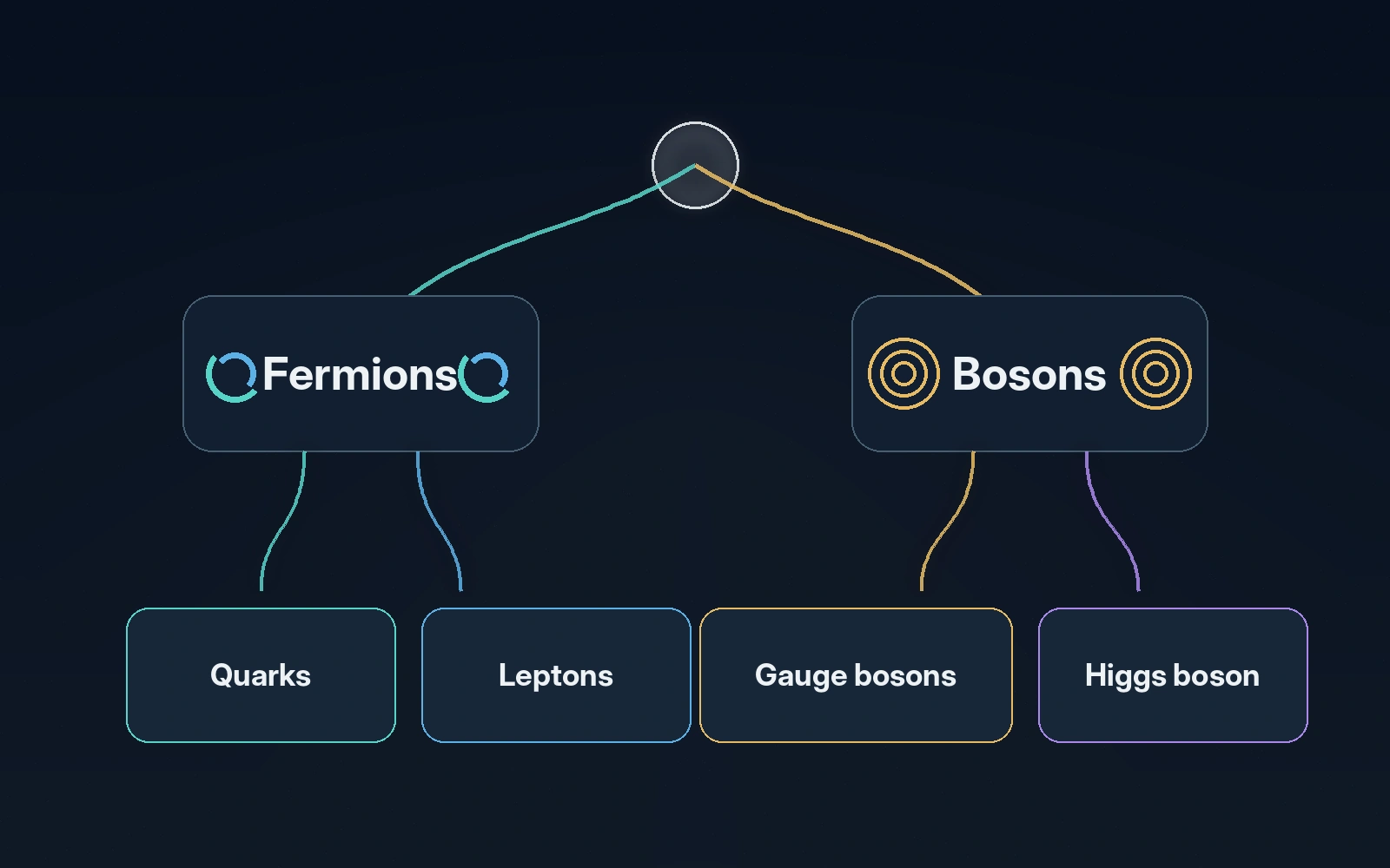
Caption: The first major classification of elementary particles follows their spin and quantum statistics: fermions include quarks and leptons, while bosons include gauge bosons and the Higgs boson.
Quantum states, kets, and complex vector spaces
A pure quantum state is represented abstractly by a ket:
The symbol denotes a vector in a complex Hilbert space, which is a complex vector space equipped with the additional structure needed to define lengths, angles, and probabilities. The ket is the state of the system in abstract form. It is not itself a measurement result, an observable, or an operator.
More precisely, multiplying a normalized ket by an overall complex phase does not change the physical pure state. For the present discussion, however, it is sufficient to work directly with normalized ket vectors.
A ket becomes a column of coordinates only after a basis has been chosen. The same abstract state can therefore have different coordinate columns in different bases, just as an ordinary geometric vector can have different components when expressed relative to different coordinate axes.
Consider a two-dimensional quantum system, often called a qubit. Choose the computational basis
In this selected basis, the two basis states are represented by the coordinate columns
These columns answer a simple coordinate question. The first column says “one unit of the first basis state and none of the second.” The second says “none of the first basis state and one unit of the second.”
A general normalized state of the same two-dimensional system can be written as
where
and normalization requires
Here, and are generally complex probability amplitudes. If the system is measured in this basis, is the probability associated with the first basis state and is the probability associated with the second.
Several distinctions are essential:
- and are basis vectors, not numerical measurement values;
- and are amplitudes, not measurement outcomes;
- and are probabilities in this selected basis;
- the basis contains two independent elementary directions, not every possible state of the qubit;
- infinitely many normalized states can be formed from complex linear combinations of these two basis states.
The elements of a basis are therefore the fundamental states relative to which the system is represented. The word “fundamental” here does not mean “fundamental particle.” It means only that the selected basis states are the independent reference directions used to express every state in that space. Before measurement, the system may occupy any of infinitely many states obtained as complex linear combinations of those basis states, each multiplied by its own complex amplitude.
Basis states, arbitrary states, and possible measurement results
It is easy to confuse the number of basis vectors with the number of states available to the system. A two-dimensional state space has two vectors in any basis, but it contains infinitely many possible state vectors. The coefficients and can vary continuously, subject to normalization and the physical irrelevance of an overall phase.
A measurement question is more specific. Once an observable has been selected, that observable has a definite set of possible measurement values. Its eigenstates provide a natural basis in which to express the system’s state. A measurement returns one of the observable’s eigenvalues; it does not normally return an arbitrary value between them.
For example, if
is measured in the computational, or , basis, the measurement selects one of the two basis eigenstates. The numerical outcomes associated with the Pauli observable are and , whereas and are the corresponding state vectors. In quantum computing, the same states are conventionally labelled with the classical symbols and , but those labels should not be confused with the physical eigenvalues of .
The system occupies a state. The observable does not “occupy a superposition.” Instead, the observable is represented by an operator that acts on the state.
Operators, observables, and the hat notation
An operator acting on quantum states is commonly written with a hat, for example
The hat signals that is an operator. It does not, by itself, guarantee that the operator represents an observable or that it has any particular symmetry property.
A physical observable is represented by a Hermitian operator. Hermiticity means
where the dagger denotes the conjugate transpose in a matrix representation. This condition guarantees that the eigenvalues of the observable are real, as physical measurement results must be.
We must also distinguish the abstract operator from its matrix representation. The operator is the basis-independent transformation acting on states. After a basis is selected, that operator is represented by a matrix whose entries depend on the chosen basis.
When a ket is written as a column vector, the operator matrix acts from the left:
This equation says that applying the operator to the input state produces another state . The state vector is not itself an operator, and its entries are coordinates of the state in the chosen basis.
Eigenvectors in linear algebra and eigenstates in quantum mechanics
The ordinary eigenvalue equation of linear algebra is
The question answered by this equation is: which nonzero vectors are transformed without being deflected away from their own one-dimensional direction, and by what scalar factor are they modified?
More formally, the transformed vector remains in the one-dimensional span of the original vector:
The vector must be nonzero. The scalar is its eigenvalue for the specified transformation . For real eigenvalues, the action can be visualized as follows:
- if , the vector is extended;
- if , it is contracted;
- if , it remains unchanged;
- if , its orientation is reversed and its magnitude is extended or contracted according to ;
- if , it is mapped to the zero vector.
In quantum mechanics the same algebraic relation is written
Here, is the quantum operator, is an eigenstate of that operator, and is the associated eigenvalue. If represents an observable, is a possible result of measuring that observable.
The correspondence is exact:
| Linear algebra | Quantum mechanics |
|---|---|
| matrix or linear operator | quantum operator |
| eigenvector | eigenstate $ |
| eigenvalue | possible measurement result , when is an observable |
| vector space | complex Hilbert space |
Quantum mechanics does not replace the logic of ordinary linear algebra. It applies the same logic in complex vector spaces and assigns physical meaning to the vectors, operators, and eigenvalues. Quantum states and eigenvectors may have complex components. A generic linear operator may also have complex eigenvalues. Hermitian observable operators, however, have real eigenvalues.
An eigenvector is never an eigenvector “of the vector space” by itself. It is always an eigenvector of a specified transformation acting on that space. Likewise, an eigenvalue is not an intrinsic property of a vector independently of the operator.
If
then every nonzero scalar multiple of is also an eigenvector with the same eigenvalue, because
Therefore, one eigenvalue does not generally correspond to only one eigenvector. The complete set of vectors associated with the same eigenvalue, together with the zero vector, forms an eigenspace:
Here, denotes the eigenspace, is the identity transformation, and the equation selects every vector left within the same direction and scaled by . Depending on the operator, an eigenspace may be a line through the origin, a plane, or a higher-dimensional subspace. For a nondegenerate two-dimensional Hermitian operator, each eigenvalue commonly has a one-dimensional eigenspace, but this is not a universal one-to-one rule.
Deriving the characteristic equation
The usual procedure for finding eigenvalues begins with
Move both terms to the same side:
Because multiplying by the scalar is equivalent to applying , we have
Therefore,
This homogeneous system must possess a nonzero solution, because an eigenvector cannot be the zero vector. If were invertible, multiplying both sides by its inverse would force
which is forbidden for an eigenvector. Consequently, must be non-invertible, and for a finite square matrix this requires
This is the characteristic equation. Its solutions are the eigenvalues of . The order of calculation is therefore
After each eigenvalue has been found, it is substituted into
in order to determine the associated eigenspace and then choose normalized eigenvectors. The eigenvalue is not substituted back into the determinant equation to obtain an eigenvector; it is substituted into this homogeneous matrix equation.
Complete example: deriving the eigenstates of Pauli
The Pauli operator is represented in the computational basis by
We begin without assuming its eigenstates. Let a generic complex state vector be
We seek the nonzero states for which applying changes only the overall scalar:
Equivalently,
with
The characteristic equation is
A product is zero when at least one factor is zero, so
Therefore the two eigenvalues are
These are the possible numerical outcomes of measuring the Pauli observable.
Eigenstate associated with
Substitute into the homogeneous equation:
This gives
Multiplying the matrix by the column produces the equations
Thus , while is free. Every vector in this eigenspace has the form
The eigenspace is the complex line generated by . Choosing the normalized representative gives
and direct substitution confirms
Eigenstate associated with
Now substitute :
This gives
The resulting equations are
Thus , while is free. Every vector in this eigenspace has the form
Choosing the normalized representative gives
and therefore
Starting only from the Pauli matrix, the ordinary eigenvalue procedure of linear algebra therefore produces the eigenvalues and , their two eigenspaces, and the normalized quantum eigenstates and .
Why diagonal matrices make the result easy to see
A diagonal matrix has the form
When an operator is represented by a diagonal matrix in a selected basis, each basis vector is an eigenvector, and the corresponding diagonal entry is its eigenvalue:
The off-diagonal entries vanish, so the operator acts independently on each basis direction instead of mixing one basis direction into another. The entries of the main diagonal can therefore be read directly as eigenvalues when the operator is represented by a diagonal matrix in the selected basis. The diagonal entries of an arbitrary non-diagonal matrix are not automatically its eigenvalues.
The Pauli matrix is already diagonal in the computational basis. Its eigenvalues and eigenvectors are therefore visible immediately, although deriving them explicitly shows why the result follows from the general procedure rather than from a special quantum rule.
Eigenstates and measurement probabilities
If a system is already in an eigenstate of an observable,
then measuring returns the value with certainty. The state is already aligned with one of the directions that the observable does not mix with the others.
For a general state expanded in an orthonormal eigenbasis,
denotes an eigenstate, is its eigenvalue, and is the amplitude of that component. The possible measurement results are the eigenvalues , and their probabilities are
For Pauli ,
so the possible results are
with probabilities
If the same two-state mathematics describes physical spin measured along the -axis, the spin operator is
The eigenstates remain and , but the physical spin values become
This is a direct example of one abstract state-space structure supporting a specific physical observable once the operator and its units are identified.
From one quantum system to several
A single ket describes one quantum system. When two systems must be described jointly, their state spaces are combined with the tensor product, written .
If one subsystem is in and another is in , their product state is
The subscripts and label the two formal subsystem slots; they are not numerical coefficients. The tensor product creates the joint state space in which both parts can be represented together. It is different from adding kets, which creates a superposition within a state space. A more explicit coordinate construction will be developed later when colour states are combined.
With this language in place, the exchange symmetry of identical particles can be stated without treating and as mysterious symbols detached from an underlying state.
Identical particles and exchange symmetry
Suppose two identical quantum particles have available one-particle states and . For fermions, the antisymmetric two-particle state is
when and are distinct orthonormal states. The first term assigns state to the first formal slot and state to the second; the second term exchanges the assignments. The minus sign makes the complete state antisymmetric under exchange.
If the two one-particle states were identical, so that , the antisymmetrized expression would become
The two terms cancel exactly. The attempted configuration has zero amplitude and therefore zero probability. Because the zero vector cannot be normalized into a physical state, no valid two-fermion state exists in which both identical fermions occupy the same complete one-particle state.
The same joint state can be represented in position space by a wavefunction , where and stand for the coordinates and any other labels needed to specify the two formal slots. The wavefunction is not a different physical object; it is a coordinate representation of the abstract joint ket.
For identical fermions, exchange antisymmetry is written
For identical bosons, the joint state is symmetric:
Because the particles are truly identical, exchanging their formal labels cannot produce a new physically distinguishable arrangement. The mathematical state may nevertheless preserve its sign, as for bosons, or acquire a minus sign, as for fermions.
The minus sign for fermions has the profound consequence just derived. If two identical fermions were placed in exactly the same complete one-particle state, exchanging them would change nothing in the written configuration, yet antisymmetry would require the state to equal its own negative. The only possible vector is the zero vector.
This is the Pauli exclusion principle: two identical fermions cannot occupy the same complete quantum state.
Electrons in atoms are therefore forced to occupy different combinations of orbital and spin states. This creates atomic shell structure, the organization of the periodic table, and much of the stability and diversity of ordinary matter.
Bosons do not obey this exclusion rule. Many identical bosons can occupy the same quantum state. This possibility underlies phenomena such as lasers, in which many photons occupy a highly coherent set of modes, and Bose-Einstein condensates, in which many atoms collectively behave as a shared quantum system.
The statement that fermions “build matter” and bosons “carry forces” is a useful first approximation, but it is not an absolute definition. Composite particles can be fermions or bosons depending on their total spin. Moreover, the Higgs boson is not a force carrier in the same sense as a photon or gluon. The deeper distinction is the spin-statistics relation and the corresponding exchange symmetry.
Quantum mechanics therefore preserves the mathematical logic of linear algebra while assigning it a physical interpretation. Quantum states are complex vectors, operators are linear transformations, and the eigenstates of an observable are the state-space directions that the operator does not mix with other directions. The associated eigenvalues are the possible results of measuring that observable. The characteristic equation determines those values, while the corresponding homogeneous systems determine their eigenspaces and normalized eigenstates. The tensor product then extends the same vector-space structure from individual systems to composite quantum systems.
This bridge now allows the particle-physics discussion to proceed with sharper language. Quarks and leptons are fermionic field excitations; their states carry quantum numbers; several constituents require a joint tensor-product space; and the symmetry of the complete state constrains which composite arrangements can physically exist.
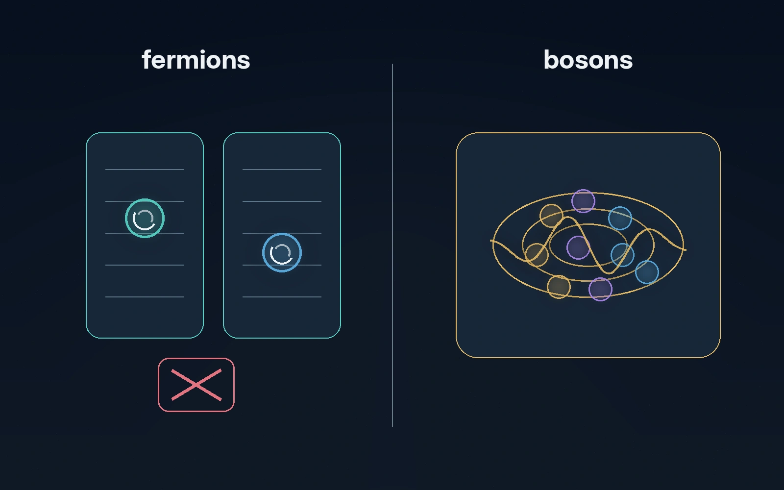
Caption: The diagram is schematic: identical fermions cannot occupy the same complete quantum state, whereas many identical bosons can share one state.
Fermions: Quarks and Leptons
The elementary fermions of the Standard Model are divided into quarks and leptons. They appear in three generations.
Each generation follows the same broad structural pattern but contains particles of increasing mass. Ordinary stable matter is built almost entirely from first-generation fermions. The heavier generations are produced in energetic processes and then decay into lighter particles.
| Generation | Quarks | Charged lepton | Neutral lepton |
|---|---|---|---|
| First | up, down | electron | electron neutrino |
| Second | charm, strange | muon | muon neutrino |
| Third | top, bottom | tau | tau neutrino |
The three charged leptons all have electric charge in units where the proton has charge . The three neutrinos have zero electric charge. Quarks carry fractional electric charges: up-type quarks have charge , while down-type quarks have charge .
Thus the up, charm, and top quarks carry charge , while the down, strange, and bottom quarks carry charge .
Leptons
The electron is the most familiar lepton. It participates in electromagnetic and weak interactions but not in the strong interaction.
The muon and tau have the same electric charge and spin as the electron but are more massive. They are unstable and eventually decay into lighter particles.
Each charged lepton is associated with a neutrino: the electron neutrino, muon neutrino, and tau neutrino. Neutrinos have no electric charge and interact through the weak interaction and gravity. Their weak interactions make them extremely difficult to detect, so vast numbers can pass through ordinary matter without leaving a measurable signal.
Neutrinos are not simply passive or massless particles. Experiments show that neutrinos produced with one flavour can later be detected with another. This phenomenon, called neutrino oscillation, requires the propagating neutrino states to have different masses.
The minimal original formulation of the Standard Model treated neutrinos as massless. Neutrino oscillations therefore demonstrate that this minimal formulation is incomplete. They do not, by themselves, uniquely determine the deeper mechanism responsible for neutrino mass.
Quarks
Quarks participate in the strong, weak, and electromagnetic interactions. Unlike leptons, they carry colour charge.
The six quark flavours are:
- up;
- down;
- charm;
- strange;
- top;
- bottom.
Up and down quarks form the dominant valence content of protons and neutrons. Strange, charm, bottom, and top quarks appear in unstable particles or high-energy reactions. The top quark is so short-lived that it decays before it can form an ordinary hadron.
Quarks are not observed as isolated free particles. They are confined inside colour-neutral composite states. To understand this statement accurately, flavour and colour must be kept conceptually separate.
Flavour, colour, confinement, and composite states
Quark flavour is the species label distinguishing up, down, charm, strange, top, and bottom quarks. Different flavours have different masses, electric charges, and weak-interaction behaviour. Flavour is not a colour label.
Colour charge is a separate quantum number belonging to quantum chromodynamics, or QCD, the quantum field theory of the strong interaction. The conventional colour labels are red, green, and blue, with corresponding anticolours for antiquarks. These words are mathematical names. They have nothing to do with visible colours or electromagnetic light.
It is also misleading to imagine that a confined quark possesses one permanently observable classical colour hidden inside a hadron. Colour is a quantum degree of freedom. The colour assigned to an individual confined quark is not, by itself, a gauge-invariant observable. What is physically meaningful is the gauge-invariant structure of the complete state.
Observable hadrons must be colour singlets: their combined colour state is neutral under the colour symmetry of QCD. The colour part of a hadron’s joint quantum state is generally a superposition, not a classical arrangement of independently inspectable coloured objects.
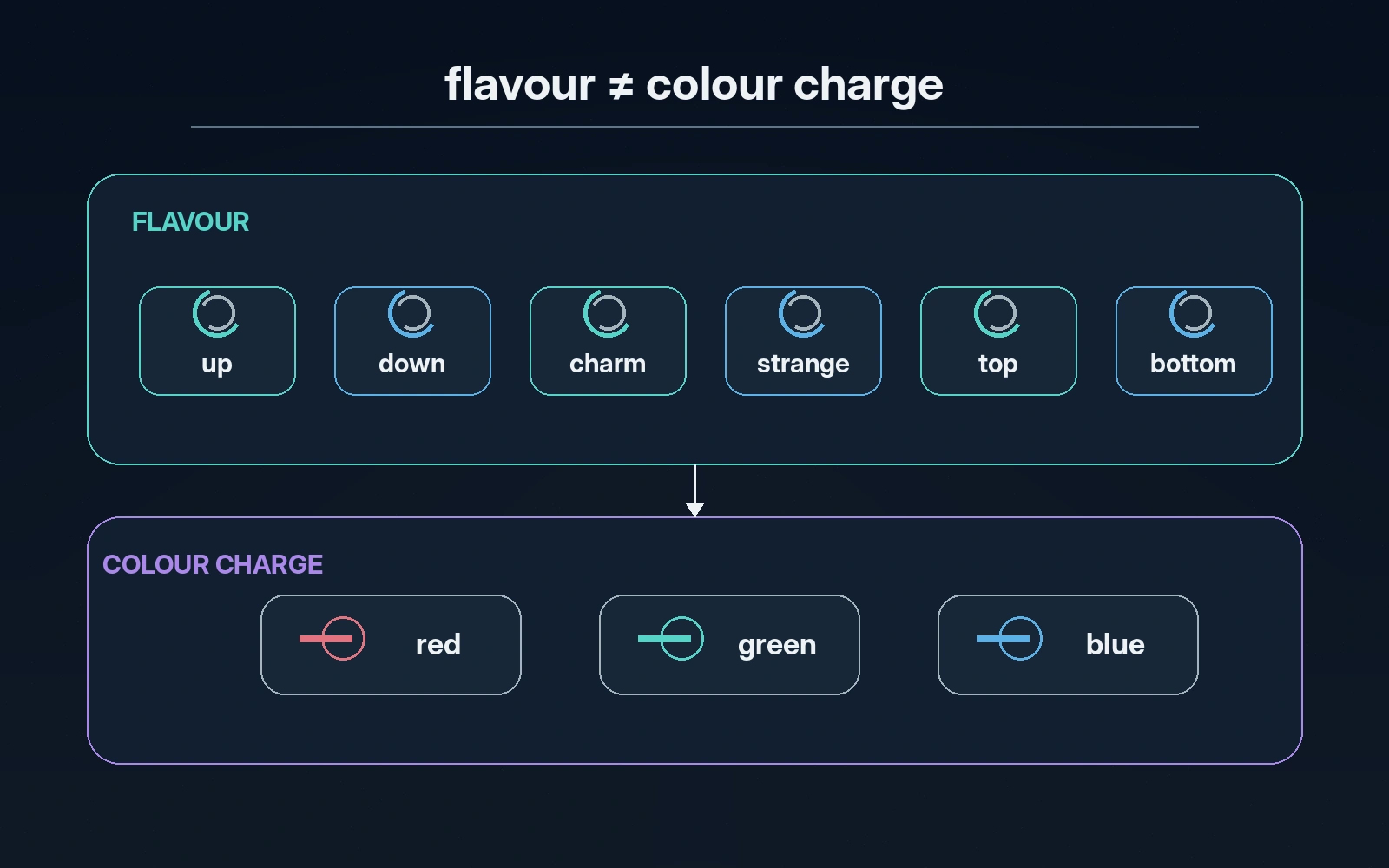
Caption: Flavour identifies a quark species, whereas colour charge is a distinct quantum number governing the strong interaction.
What the tensor product actually constructs
The tensor-product symbol
combines the state spaces of distinct subsystems or degrees of freedom. It is not scalar multiplication, an inner product, a vector cross product, ordinary matrix multiplication, or an enumeration of permutations.
The contrast with ordinary matrix multiplication is important. Matrix multiplication combines rows and columns and produces sums of products. For example,
The first output component is the sum , and the second is the sum . This operation applies a linear transformation to a vector.
The tensor product of two vectors performs a different construction. Let
Their tensor product is
No row-column sums are formed. Every ordered product of a component from the first vector with a component from the second is retained separately. The tensor product thereby constructs all ordered combinations of the basis states of the two subsystems.
If the first state space has dimension and the second has dimension , the composite state space has dimension
For two qubits,
Each qubit requires two coordinates, while the pair requires four coordinates because there are four ordered joint basis states.
From a coordinate column to a composite ket
Use the one-qubit basis vectors
Their tensor product gives
To interpret this column, choose the conventional ordered basis
The four basis kets have the coordinate representations
When a coordinate column in this composite basis contains only zeros except for one entry equal to , the position of that identifies the selected basis vector. The column selects the second vector in the ordered basis, namely :
The column vector is not physically transformed into the ket by another operation. They are two representations of the same state:
- is the abstract Dirac notation;
- is its coordinate representation in the selected ordered basis.
The ordering of the composite basis is a convention. A different consistent ordering would assign the coordinate positions differently, so the chosen order must remain fixed throughout a calculation.
Each compact composite ket also abbreviates a tensor product:
The first label refers to the first subsystem slot and the second label to the second subsystem slot.
Tensor composition is not superposition
The symbols and perform fundamentally different roles. A sum forms a superposition within a state space:
A tensor product combines distinct subsystems:
If
and
then distributivity gives
The tensor product first constructs the composite space. The plus signs then form a superposition of its composite basis states. The four coefficients , , , and are the amplitudes associated with the four ordered joint configurations.
This example uses qubits only because their coordinates are easy to display. The same structural logic applies whenever quantum subsystems are combined, including colour degrees of freedom. The dimensions, basis labels, and physical interpretation change, but the tensor-product operation continues to build the joint space.
Applying the tensor product to meson colour
A quark transforms in the three-dimensional colour representation, written , while an antiquark transforms in the corresponding conjugate representation, written . The tensor product
constructs the joint colour-representation space of the quark and antiquark. This composite space can then be decomposed into invariant sectors:
The symbols and describe different operations. The tensor product builds the composite representation space. The direct sum states that this space can be separated into distinct invariant representation sectors. The direct sum is not a quantum superposition and does not mean that particles are being added.
The is the colour-singlet sector. A quark-antiquark state in this sector can correspond to a physically observable colour-neutral meson. The is a non-singlet colour sector and cannot describe an isolated observable hadron.
Schematically, the colour-singlet state of an ordinary meson is
Each ket, such as , abbreviates a tensor product between a quark colour basis state and an antiquark anticolour basis state. The plus signs form a coherent superposition of three joint basis states, and normalizes the state when those basis states are orthonormal.
This expression does not say that the meson is sometimes red-antired, sometimes green-antigreen, and sometimes blue-antiblue in an ordinary classical sense. It describes one quantum state whose complete colour structure belongs to the neutral singlet sector.
Applying the tensor product to baryon colour
For three quarks, the colour representations combine according to
The tensor products on the left build the full joint colour space of three quark constituents. The direct sums on the right decompose that space into one singlet sector, two octet sectors, and one decuplet sector.
The is the colour-singlet component corresponding to an observable colour-neutral baryon. The two sectors and the sector are non-singlet representations.
The normalized colour-singlet state can be written schematically as the antisymmetric combination
Each three-letter ket abbreviates a threefold tensor product, for example
The six terms include every ordering of red, green, and blue. Their signs make the colour factor antisymmetric under exchange of any two colour slots. This antisymmetry is not merely decorative: it participates in ensuring that the complete state of identical quarks has the fermionic exchange behaviour required by the Pauli principle. The full baryon state also includes spatial, spin, and flavour factors, so the symmetry of the total state depends on how all these parts combine.
The usual valence structures are:
- a baryon contains three valence quarks;
- a meson contains one valence quark and one valence antiquark.
“Valence” does not mean that the interior contains only those particles. A hadron is a dynamical QCD system containing gluon fields and continuously fluctuating quark-antiquark contributions, often described as the sea. The valence content identifies the quantum numbers that remain after these additional contributions are accounted for.
QCD also permits exotic colour-neutral combinations. Experimentally observed tetraquark candidates contain a valence structure involving two quarks and two antiquarks, while pentaquark candidates involve four quarks and one antiquark. Their internal organization may be compact, molecular, or a quantum mixture of configurations, depending on the state. Whatever their detailed structure, the complete physical hadron must remain colour-neutral.
The fact that isolated quarks are not detected is called colour confinement. At very short distances, the strong interaction can become comparatively weak, a property known as asymptotic freedom. As quarks are pulled apart, however, the colour field does not spread and fade in the same way as the electric field between separated charges. The energy stored in the colour field grows until it becomes favourable to create new quark-antiquark pairs. The result is not a free quark but additional colour-neutral hadrons.
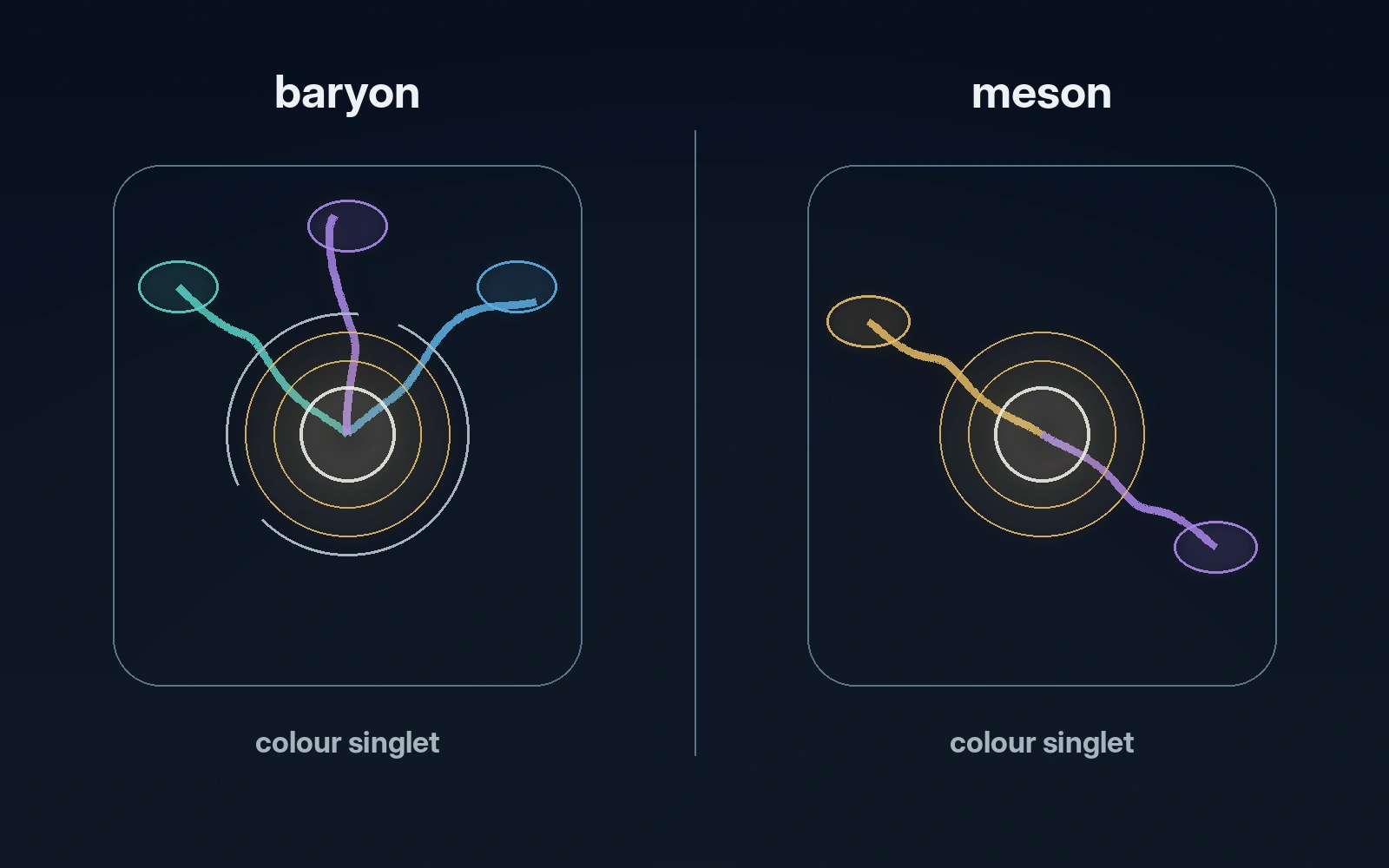
Caption: Ordinary baryons have three valence quarks and ordinary mesons have a valence quark-antiquark pair; in both cases, the complete physical hadron is colour-neutral.
Antimatter
Every elementary fermion has a corresponding antiparticle with the same mass and spin but opposite additive charges.
The antiparticle of the electron is the positron, which has electric charge . An antiquark has the electric charge opposite to that of its corresponding quark and transforms in the anticolour representation. Neutrinos also have corresponding antineutrino states, although the deeper question of whether neutrinos are distinct from their own antiparticles remains experimentally unresolved.
Antimatter is not matter with negative mass, nor does it necessarily move backward through ordinary time. It is described by quantum fields whose particle and antiparticle excitations carry opposite relevant quantum numbers.
When a particle and its antiparticle annihilate, their energy and conserved quantum numbers are transferred into other excitations. Electron-positron annihilation can, for example, produce photons. Conversely, sufficiently energetic photons or other interactions can create particle-antiparticle pairs.
The observable universe contains far more matter than antimatter. The known differences between matter and antimatter in Standard Model processes do not appear sufficient to explain this cosmic imbalance fully.
Bosons: Interactions and the Higgs Field
Elementary bosons in the Standard Model fall into two conceptual groups:
- gauge bosons associated with the electromagnetic, strong, and weak interactions;
- the Higgs boson, which is the excitation of the Higgs field.
The established gauge bosons are the photon, eight gluons, the two charged bosons, and the neutral boson.
The photon
The photon is the quantum of the electromagnetic field. It is massless, has spin , and mediates electromagnetic interactions between electrically charged particles.
In quantum field theory, “mediation” does not mean that classical particles simply throw tiny photon pellets at one another. Interactions are encoded through couplings between quantum fields. The language of exchanged virtual particles can be useful in perturbative calculations, but virtual particles are internal mathematical elements of those calculations, not directly detectable particles travelling along ordinary trajectories.
The photon itself carries no electric charge, so electromagnetic fields do not directly self-interact in the same way that gluon fields do. Quantum effects can nevertheless allow indirect photon-photon interactions through electrically charged fields.
Gluons
Gluons are the gauge bosons of QCD. There are eight independent gluon states, and they are massless in the Standard Model.
Unlike photons, gluons carry colour charge. They therefore interact with quarks and with other gluons. This self-interaction is central to the complexity of QCD, the confinement of quarks, and the internal dynamics of hadrons.
A proton is consequently not well described as three static quarks sitting inside a container. It is a relativistic quantum state of quark and gluon fields. Its three valence quarks determine key quantum numbers, but gluons and sea quark-antiquark fluctuations contribute essentially to its structure.
The and bosons
The weak interaction is mediated by the charged and bosons and the neutral boson. These particles are massive and have spin .
Weak interactions can transform one fermion flavour into another. In beta decay, for example, the process can be described at the quark level as a down quark transforming into an up quark while producing a virtual that leads to an electron and an antineutrino.
Because the and bosons are heavy, the weak interaction has a very short effective range at ordinary energies. It plays a central role in radioactive decay, neutrino interactions, stellar processes, and the transformation of particle species.
The weak interaction also distinguishes between left- and right-handed structures in a fundamental way. This violation of mirror symmetry is one of its most striking properties.
The Higgs field and Higgs boson
The Higgs field is a scalar quantum field whose vacuum state has a nonzero value throughout empty space. Through their interactions with this field, the and bosons acquire mass while the photon remains massless.
Fermions can also acquire masses through their couplings to the Higgs field. Different coupling strengths correspond to different fermion masses, although the Standard Model does not explain why these couplings take their observed numerical values.
The Higgs boson is the observable quantum excitation associated with disturbances of the Higgs field. It has spin and was discovered in 2012 through experiments at CERN’s Large Hadron Collider.
It is inaccurate to say that the Higgs field “creates all mass.” The Higgs mechanism is essential for the masses of elementary fermions and the weak gauge bosons, but most of the mass of protons and neutrons does not come directly from the bare masses of their quarks.
Most nucleon mass arises from QCD dynamics: the energy of confined quark and gluon fields, their motion, and the strong interaction itself. Through the mass-energy relation, this internal energy contributes to the proton’s and neutron’s mass.
The visible mass of ordinary objects is therefore largely a manifestation of strong-interaction energy, even though the Higgs field remains indispensable to the structure of the Standard Model.
Composite Particles: Hadrons, Nuclei, and Ordinary Matter
Particles composed of quarks and gluons are called hadrons. The two most familiar classes are baryons and mesons.
A proton is a baryon with valence quark content : two up quarks and one down quark. Their electric charges combine as
A neutron is a baryon with valence quark content . Its valence charges combine as
These formulas correctly reproduce the total electric charges, but they should not be mistaken for a complete model of nucleon structure. Protons and neutrons are extended quantum systems governed by QCD.
Mesons contain a valence quark and antiquark. They are generally unstable and play important roles in nuclear interactions and particle decays.
Protons and neutrons bind together to form atomic nuclei. The force between nucleons is a residual effect of QCD, somewhat analogous in spirit to how neutral atoms can still exert electromagnetic forces on one another even though their total electric charge is zero. Nuclear forces are not produced by freely exchanging gluons between colour-neutral protons and neutrons in a simple classical manner; they emerge from the underlying strong dynamics of composite hadrons.
Electrons bind to nuclei through electromagnetism, forming atoms. Atoms combine into molecules, solids, liquids, living cells, planets, and stars.
The macroscopic world is therefore not built merely by placing elementary particles next to one another. It emerges from multiple layers of quantum organization:
- quantum fields permit particle excitations;
- fermionic statistics generate stable matter structures;
- gauge interactions bind and transform particles;
- QCD creates hadrons;
- electromagnetism creates atoms and chemistry;
- collective behaviour produces macroscopic materials.
The Standard Model as a Quantum Field Theory
The Standard Model is often presented as a chart of particles. The chart is useful, but it is not the theory itself.
The Standard Model is a relativistic quantum field theory that specifies:
- which fundamental fields exist;
- how those fields transform under symmetries;
- which interactions are permitted;
- how particles acquire mass through electroweak symmetry breaking;
- how probabilities for scattering and decay processes can be calculated.
Its internal organization is summarized by the gauge symmetry
This notation should not be treated as a decorative formula.
The factor organizes the colour symmetry of QCD. It determines the structure of the strong interaction, including the existence of eight gluons and their couplings to quarks and to one another.
The factors and organize the electroweak theory, which unifies the mathematical description of electromagnetic and weak interactions before electroweak symmetry breaking. The subscript reflects the special role of left-handed fermion fields, while denotes weak hypercharge.
The Higgs field changes how the electroweak symmetry appears in the vacuum. After symmetry breaking, the underlying electroweak fields reorganize into the observed photon, , , and bosons. The photon remains massless, while the weak bosons become massive.
Gauge symmetry is not merely a way to sort particles into boxes. It constrains the possible interactions. Once the fields and symmetry structure are specified, many couplings and conservation rules follow from the theory’s mathematical consistency.
The Standard Model has achieved extraordinary experimental success. It predicts particle properties, scattering rates, decay probabilities, and quantum corrections with remarkable precision. Measurements of the electron’s magnetic properties, electroweak processes, collider events, and strong-interaction phenomena have repeatedly confirmed its structure.
Yet its success does not make it a complete theory of nature.
A Compact Map of the Elementary Particles
The established elementary particle content can be summarized as follows:
| Class | Members | Spin | Main role |
|---|---|---|---|
| Quarks | up, down, charm, strange, top, bottom | Colour-charged fermions; constituents of hadrons | |
| Charged leptons | electron, muon, tau | Electrically charged fermions not subject to the strong interaction | |
| Neutrinos | electron, muon, tau neutrinos | Electrically neutral fermions participating in weak interactions | |
| Gauge bosons | photon, eight gluons, , , | Quanta associated with electromagnetic, strong, and weak gauge fields | |
| Higgs boson | Higgs boson | Excitation of the Higgs field |
Antiparticles accompany the fermions, and the charged bosons are antiparticles of one another. The photon and boson are their own antiparticles. Gluon antiparticle relations are encoded within the gluon colour structure rather than through eight separate additional antiglue particles.
This table summarizes the field excitations considered elementary by the Standard Model. It does not include composite hadrons, atomic nuclei, atoms, or hypothetical particles not yet experimentally established.
The Four Fundamental Interactions
Physics commonly speaks of four fundamental interactions: electromagnetism, the weak interaction, the strong interaction, and gravity. This list is useful, but it hides an important asymmetry. The first three are described within the Standard Model. Gravity is not.
Electromagnetism
Electromagnetism acts on electrically charged particles and is associated with the photon. It has infinite range because the photon is massless, although neutral systems can screen or suppress electromagnetic effects at large distances.
Electromagnetism governs atomic binding, chemistry, light, electricity, magnetism, and most of the contact forces encountered in daily life.
The weak interaction
The weak interaction acts on quarks and leptons and is associated with the and bosons. It can change particle flavour and is responsible for processes such as beta decay.
Its short effective range results from the large masses of the weak bosons. Together with electromagnetism, it forms the electroweak sector of the Standard Model.
The strong interaction
The strong interaction acts on colour charge and is described by QCD. Its gauge bosons are gluons.
At the level of quarks and gluons, the strong interaction produces confinement and asymptotic freedom. At the level of protons and neutrons, residual strong effects help bind atomic nuclei.
Calling it simply “the force that holds the nucleus together” is therefore incomplete. Its more fundamental role is to govern colour-charged quantum fields and to generate hadrons themselves.
Gravity
Gravity acts on energy and momentum and dominates the large-scale structure of planets, stars, galaxies, and the universe.
The best established classical theory of gravity is general relativity, which describes gravity as the geometry of spacetime rather than as an ordinary force field propagating on a fixed background.
Gravity has not yet been incorporated into the Standard Model. Physicists expect that a complete description of nature must reconcile quantum theory with gravity, but no experimentally confirmed quantum theory of gravity currently exists.
A hypothetical quantum of the gravitational field is called the graviton. It is commonly expected to be a massless spin- particle in perturbative quantum descriptions of gravity. However, no graviton has been detected, and it is not an established member of the Standard Model.
What the Standard Model Does Not Yet Explain
The Standard Model is one of the most successful scientific theories ever constructed, but several observations and theoretical problems indicate that it is incomplete.
Dark matter
Astronomical and cosmological evidence shows that galaxies and larger structures behave as though they contain far more gravitating matter than can be accounted for by visible stars, gas, dust, and known Standard Model particles.
The nature of this dark matter remains unknown. It may involve one or more new particle species, but no proposed dark-matter particle has yet been conclusively detected.
Matter-antimatter asymmetry
The observable universe is dominated by matter, even though known high-energy processes can create matter and antimatter together.
The Standard Model contains mechanisms that distinguish matter from antimatter, but their known strength appears insufficient to explain the observed cosmic asymmetry. Additional physics may be required.
Neutrino masses
Neutrino oscillations show that neutrinos have nonzero masses and that flavour states are mixtures of mass states.
The minimal original Standard Model does not provide these masses. Several extensions can accommodate them, but current experiments have not yet identified the unique underlying mechanism.
Important open questions include the absolute neutrino mass scale, the ordering of the masses, and whether neutrinos are fundamentally distinct from their antiparticles.
Quantum gravity
General relativity and quantum field theory are each extraordinarily successful in their own domains, but their standard formulations are not yet unified into a complete experimentally tested theory.
The problem becomes unavoidable in regimes where both strong gravity and quantum effects matter, such as the earliest moments of the universe or the deep interior of black holes.
The pattern of masses and generations
The Standard Model contains three fermion generations, but it does not explain why there are exactly three. Nor does it explain the observed hierarchy of fermion masses and mixing parameters from a deeper principle.
The Higgs mechanism permits elementary particles to have mass, but the experimentally measured coupling strengths must still be supplied to the theory.
Physics beyond the Standard Model
“Beyond the Standard Model” is not the name of one established theory. It is a broad category for proposed extensions intended to address unexplained observations or structural puzzles.
Possible ideas include new particles, additional symmetries, expanded Higgs sectors, new neutrino interactions, composite structures, extra dimensions, or deeper unification. None of these possibilities should be treated as experimentally confirmed merely because it is mathematically attractive.
The appropriate scientific position is neither to assume that the Standard Model is final nor to declare a favourite extension correct without evidence.
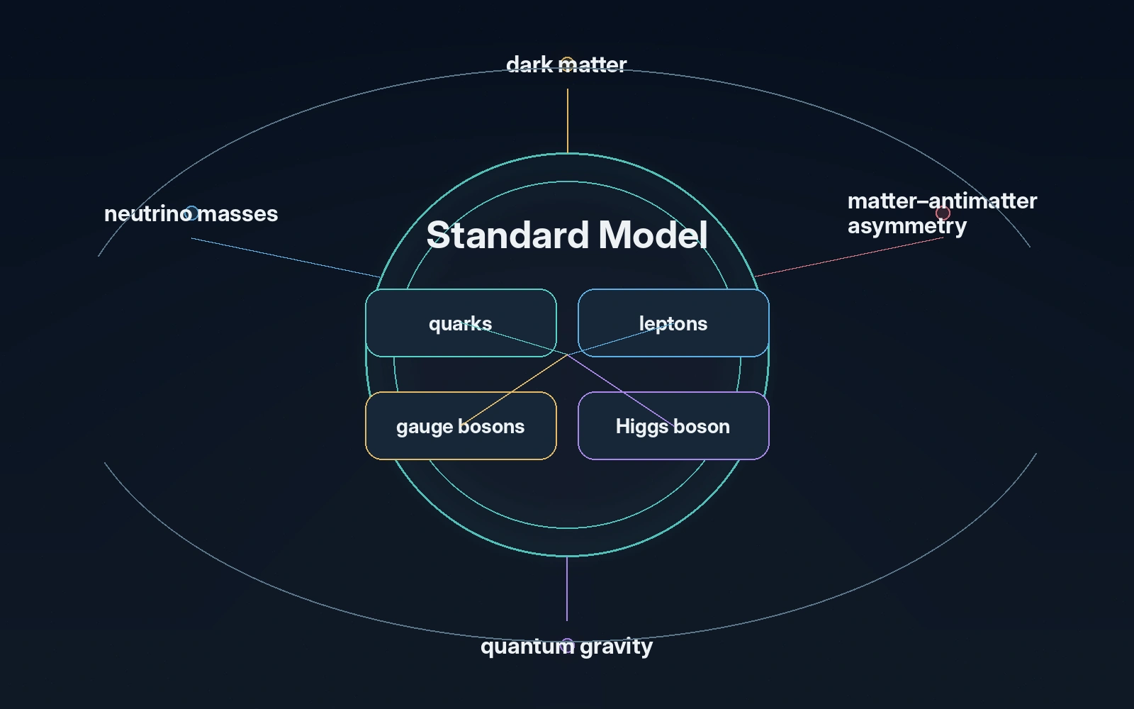
Caption: The Standard Model organizes established elementary particles and three quantum interactions, while dark matter, neutrino masses, matter-antimatter asymmetry, and quantum gravity remain open problems.
Conclusion: From Fields to the Visible Universe
A coherent understanding of fundamental particles begins not with a memorized chart but with a change in ontology.
Modern particle physics describes nature through quantum fields. What we call particles are quantized excitations of those fields, identified by properties such as mass, spin, electric charge, colour charge, and interaction behaviour.
Spin divides the elementary excitations into fermions and bosons. Fermions obey antisymmetric exchange statistics and the Pauli exclusion principle, allowing them to form the structured matter of atoms. Bosons obey symmetric statistics and include the gauge-field quanta associated with electromagnetic, strong, and weak interactions, as well as the spin-zero excitation of the Higgs field.
Quarks and leptons are the elementary fermions presently known. Quarks carry both flavour and colour, two distinct quantum properties, and are confined into colour-singlet hadrons. Protons and neutrons are therefore not elementary particles but complex QCD states whose mass arises predominantly from strong-interaction energy.
The Standard Model unites these fields and interactions through a precise symmetry structure. It explains an extraordinary range of experimental results, from particle decays to collider collisions and the quantum foundations of ordinary matter.
Yet the map remains incomplete. Gravity lies outside the Standard Model. Dark matter is unidentified. Neutrino masses require an extension of the minimal theory. The predominance of matter over antimatter remains unexplained, and the pattern of particle masses and generations still lacks a deeper account.
The visible universe can thus be understood as a layered quantum construction: fields give rise to excitations, symmetries organize their interactions, confinement produces hadrons, nuclei bind, atoms form, and collective structures emerge.
Fundamental particles are not simply the smallest objects in a box of matter. They are the experimentally accessible quantum manifestations of the fields and symmetries from which the known physical world is built.
Reader response